background-image: url("../pic/slide-front-page.jpg") class: center,middle count: false # 计量经济学II # (Econometrics II) <!--- chakra: libs/remark-latest.min.js ---> ### 胡华平 ### 西北农林科技大学 ### 经济管理学院数量经济教研室 ### huhuaping01@hotmail.com ### 2021-10-07 <div> <style type="text/css">.xaringan-extra-logo { width: 110px; height: 70px; z-index: 0; background-image: url(../pic/logo/nwafu-logo-circle-wb.png); background-size: contain; background-repeat: no-repeat; position: absolute; top:0.2em;left:1em; } </style> <script>(function () { let tries = 0 function addLogo () { if (typeof slideshow === 'undefined') { tries += 1 if (tries < 10) { setTimeout(addLogo, 100) } } else { document.querySelectorAll('.remark-slide-content:not(.title-slide):not(.inverse):not(.hide_logo)') .forEach(function (slide) { const logo = document.createElement('div') logo.classList = 'xaringan-extra-logo' logo.href = null slide.appendChild(logo) }) } } document.addEventListener('DOMContentLoaded', addLogo) })()</script> </div> --- class: center, middle, duke-orange,hide_logo name: chapter-navi count: true # 模块1：计量经济学基础 .larger[ Chapter 01. 经典模型 Chapter 02. 矩阵分析 [Chapter 03. 放宽假设](#chapter03) Chapter 04. 扩展方法 ] --- layout: false class: center, middle, duke-softblue,hide_logo name: chapter03 # 第03章 放宽假设 [3.1 多重共线性(Multi-collinearity)问题](#multi) [3.2 异方差(hetro-scadasticity)问题](#hetero) [3.3 自相关(auto-correlation)问题](#auto) [.red[3.4 内生自变量(endogeneity-variable)问题]](#endogeneity) --- layout:false background-image: url("pic/chapter-03-frame-relax.png") background-size: cover class: inverse,center <!---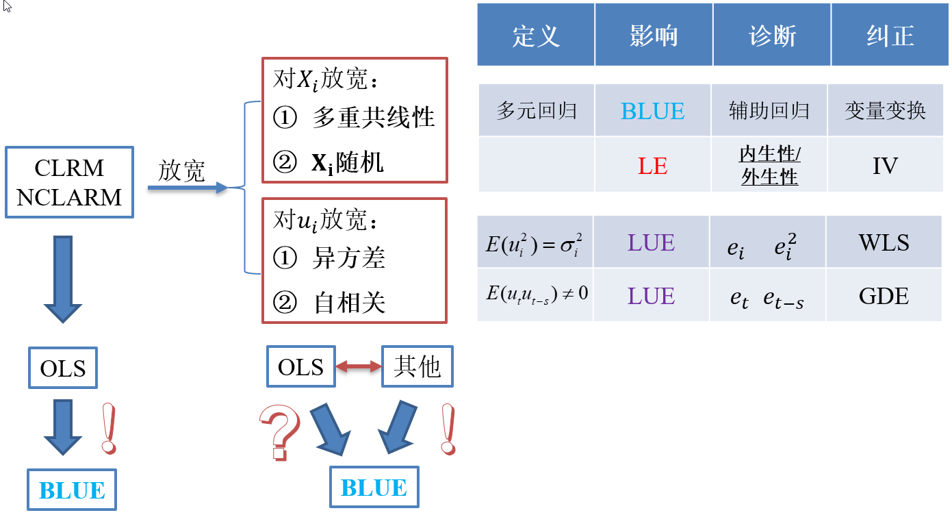---> --- layout: false class: center, middle, duke-softblue,hide_logo name: endogeneity # 3.4 内生性自变量问题 [3.4.1 内生自变量问题的定义和来源](#source) [3.4.2 内生变量法下的估计问题](#problem) [3.4.3 工具变量及其选择](#IV) [3.4.4 两阶段最小二乘法（2SLS）](#TSLS) [3.4.5 检验工具变量的有效性(Instrument validity)](#validity) [3.4.6 检验自变量的内生性(regressor endogeneity)](#endogeneity-test) --- layout: false class: center, middle, duke-softblue,hide_logo name: source # 3.4.1 内生自变量问题的定义和来源 --- layout: true <div class="my-header-h2"></div> <div class="watermark1"></div> <div class="watermark2"></div> <div class="watermark3"></div> <div class="my-footer"><span>huhuaping@ <a href="#chapter-navi">模块01 计量经济学基础 |</a> &emsp;&emsp;&emsp;&emsp; <a href="#chapter03">第03章 放宽假设 |</a> &emsp;&emsp;&emsp;&emsp; <a href="#endogeneity"> 3.4 内生性自变量（endogeneity-variable）问题 |</a> &emsp;&emsp;&emsp;&emsp; <a href="#source"> 3.4.1 内生自变量问题的定义和来源 </a> </span></div> --- ## 知识回顾 对于总体回归模型： `$$\begin{align} Y_i &= \beta_1 +\beta_2X_i + u_i && \text{(PRM)} \end{align}$$` - 在CLRM假设下：**CLRM假设A2**——X是固定的（给定的）或独立于误差项。也即自变量X**不是**随机变量。此时，我们可以使用OLS方法，并得到**BLUE**。 `$$\begin{align} Cov(X_i, u_i)= 0\\ E(X_i u_i)= 0 \end{align}$$` -- - 如果违背上述假设，也即自变量X与随机干扰项相关。此时使用OLS估计将不再能得到**BLUE**，而应该采用**工具变量法**（IV）进行估计。 `$$\begin{align} Cov(X_i, u_i)= 0\\ E(X_i u_i)= 0 \end{align}$$` -- 事实上，无论 `\(X_i\)`与 `\(u_i\)`是否相关，我们都可以采用**IV法**得到**BLUE**。 --- ## 好模型的标准与外生自变量 `$$\begin{equation} \boldsymbol{y= X \beta+u} \end{equation}$$` **随机控制实验**（randomized controlled experiment）：理想情形下，自变量X的取值是随机分配变化的（**原因**），然后我们再来观测因变量Y的变化（**结果**）。 - 如果 `\(Y_i\)`和 `\(X_i\)`确实存在系统性的关系（线性关系），那么改变 `\(X_i\)`则导致 `\(Y_i\)`的相应变化。 - 除此之外的任何其他随机因素，都将放到随机干扰项 `\(u_i\)`中，它对因变量 `\(Y_i\)`的变动影响，应该是**独立于** `\(X_i\)`的影响作用的。 --- ## 好模型的标准与外生自变量 **外生自变量**（exogenous regressors）：如果自变量 `\(X_i\)`真的是如上所说的**完美的随机取值**（randomly assigned），则称之为外生自变量。更准确地，可以定义为： > **严格外生性假设**（strictly exogeneity）： `\(E\left(u_{i} \mid x_{1}, \ldots, x_{N}\right)=E\left(u_{i} \mid \mathbf{x}\right)=0\)`。 因为在**随机控制实验**，给定样本 `\(i\)`和样本 `\(j\)`，自变量的取值分别为 `\(X_i\)`和 `\(X_j\)`，它们应该是相互独立的。因此可以把上述假设进一步简化为： > **同期外生性假设**（contemporaneously exogeneity）： `\(E(u_i|X_{i})=0, \text{for } i =1, \ldots,N\)`。 ??? **同期**表示的是在同样的时间点上，或所有的截面观测单位在某个时间上获得的观测。 --- ## 大样本情况下OLS方法 在大样本情形下，上述**严格外生性假设**可以进一步转换为**同期不相关假设**： - `\(E(u_i)=0\)`，而且 - `\(\operatorname{cov}(x_i, u_i)=0\)` 因为我们可以证明（证明略），在大样本情况OLS方法下： - `\(E(u_i|X_{i})=0 \quad \Rightarrow \quad E(u_i)=0\)` - `\(E(u_i|X_{i})=0 \quad \Rightarrow \quad \operatorname{cov}(x_i, u_i)=0\)` --- ## 内生自变量问题的定义 `$$\begin{equation} \boldsymbol{y= X \beta+u} \end{equation}$$` 在经典线性回归模型假设(**CLRM**)中，我们假设所有回归元 `\(X_{i}\)`是**给定的**，且随机干扰项的条件期望为0（ `\(E(u_i|X_{i})=0\)`）。 - 回归元是**严格外生性**具有重要意义，因为理论上将表明模型的预测误差将是最小的（等于0） - 实际上，我们的这一假设要求非常高，在**随机控制实验**中要求 `\(X_{ki}\)`是**同期外生性**的 `\(E(u_i|X_{i})=0, \text{for } i =1, \ldots,N\)`。 然而，现实中，回归元 `\(X_{i}\)`可能是**随机的**；而且回归元与随机干扰项可以能是**相关的**。此时，我们称模型存在**内生自变量**（endogenous regressors）问题。正式地： - 如果自变量与随机干扰项无关，则称之为**外生变量**（ **.red[en]dogenous**） - 如果自变量与随机干扰项相关，则称之为**内生变量**（ **.red[ex]ogenous**）。 --- ## 内生自变量问题的几种情形 在应用计量经济学中，内生性通常以以下四种方式之一出现： - **遗漏变量**（Omitted variables） - **测量误差**（Measurement errors） - **自相关问题**（Autocorrelation） - **方程联立性问题**（Simultaneity） --- ### 内生自变量情形1：遗漏变量 假定假定工资水平的“真实模型”为： `$$\begin{align} Wage_{i}=\beta_{1}+\beta_{2} Edu_{i}+\beta_{3} Abl_{i}+\epsilon_{i} \quad \text{(the assumed true model)} \end{align}$$` 然而，因为个体的**能力变量** `\(Abl\)` 往往无法直接观测得到，因此我们往往不能放入到模型中，并构建了一个有偏误的模型。 `$$\begin{align} Wage_{i}=\alpha_{1}+\alpha_{2} Edu_{i}+v_{i} \quad \text{(the error specified model)} \end{align}$$` > 其中**能力变量** `\(Abl\)` 被包含到新的随机干扰项 `\(v_i\)`中，也即： `\(v_{i}=\beta_{3} abl_{i}+u_{i}\)` 显然，我们认为偏误模型中，忽略了**能力变量** `\(Abl\)`，而**受教育年数变量** `\(Edu\)`实际上又与之有相关关系。进而偏误模型中， `\(cov(Edu_i, v_i) \neq 0\)`，从而**受教育年数变量** `\(Edu\)`具有内生自变量问题。 --- <!---demo1 ommit endo begin---> ### 内生自变量情形1：遗漏变量（演示1） 下面我们对遗漏变量情形做一个整体的直观演示：  --- ### 内生自变量情形1：遗漏变量（演示1） 下面我们对遗漏变量情形做一个整体的直观演示：  --- ### 内生自变量情形1：遗漏变量（演示1） 下面我们对遗漏变量情形做一个整体的直观演示：  --- ### 内生自变量情形1：遗漏变量（演示1） 下面我们对遗漏变量情形做一个整体的直观演示：  --- <!---demo2 ommit endo begion---> ### 内生自变量情形1：遗漏变量（演示2） 具体地，遗漏变量引发内生自变量问题的直观演示如下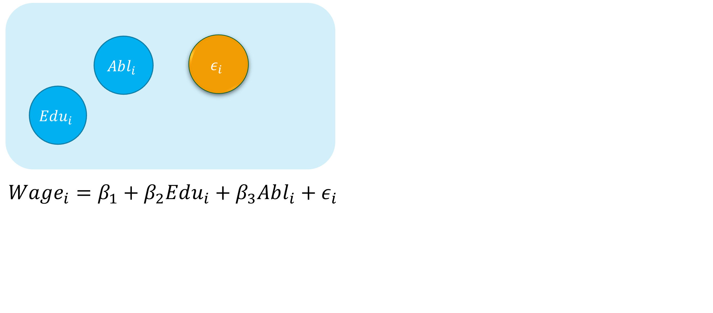：  --- ### 内生自变量情形1：遗漏变量（演示2） 具体地，遗漏变量引发内生自变量问题的直观演示如下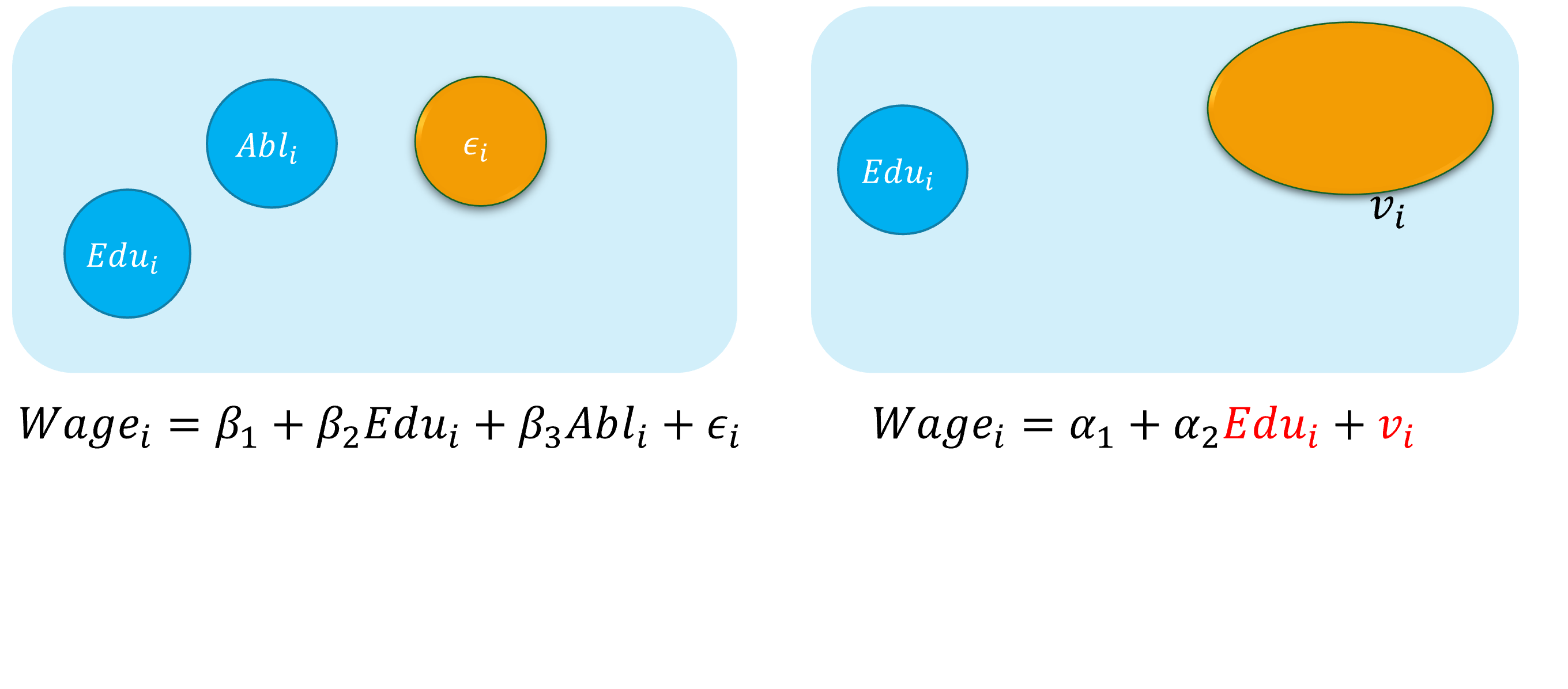：  --- ### 内生自变量情形1：遗漏变量（演示2） 具体地，遗漏变量引发内生自变量问题的直观演示如下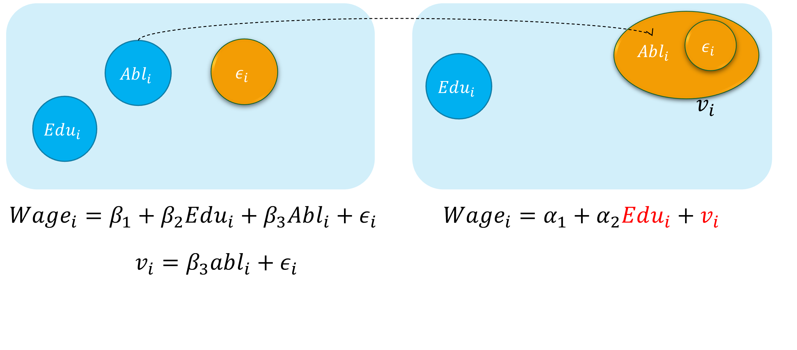：  --- ### 内生自变量情形1：遗漏变量（演示2） 具体地，遗漏变量引发内生自变量问题的直观演示如下：  --- ### 内生自变量情形1：遗漏变量（演示2） 具体地，遗漏变量引发内生自变量问题的直观演示如下：  --- ### 内生自变量情形2：测量误差 很多时候的模型中实际使用的某个自变量本身并不是准确观测的，而只是“近似物”，因此模型自变量中存在**测量误差**（measurement error）。 --- ### 内生自变量情形2：测量误差 再次, 假定工资决定的**真实模型**（real model）是： `$$\begin {align} Wage_i=\beta_{1}+\beta_{2} Edu_i+\beta_{3} Abl_i+u_i \quad \text{(the assumed true model)} \end {align}$$` 然而, 因为个体的**能力变量** `\(Abl\)` 往往无法直接观测得到，我们便会考虑使用 **智商水平** 变量 ( `\(IQ_i\)`)，并构建如下有偏误的**代理变量模型**（proxy variable model）： `$$\begin {align} Wage_i=\alpha_{1}+\alpha_{2} Edu_i+\alpha_{3} IQ_i+v_i \quad \text{(the error specified model)} \end {align}$$` - 此时，智商水平 `\(IQ_i\)`被认为是能力变量 `\(Abl_i\)`的一个**代理变量**（proxy variable）。 - 而实际上，能力水平变量 `\(Abl_i\)`的内涵要远远大于智商水平变量 `\(IQ_i\)`。因此，**受教育年数变量** `\(Edu\)`会与随机干扰项中未纳入模型的 `\(Abl_i\)`变量的测量误差部分存在相关关系。进而偏误模型中， `\(cov(Edu_i, v_i) \neq 0\)`，从而**受教育年数变量** `\(Edu\)`具有内生自变量问题。 --- <!---demo1 ommit endo begin---> ### 内生自变量情形2：测量误差（演示1） 下面我们对测量误差情形做一个整体的直观演示：  --- ### 内生自变量情形2：测量误差（演示1） 下面我们对测量误差情形做一个整体的直观演示：  --- ### 内生自变量情形2：测量误差（演示1） 下面我们对测量误差情形做一个整体的直观演示：  --- ### 内生自变量情形2：测量误差（演示1） 下面我们对测量误差情形做一个整体的直观演示：  --- <!---demo2 ommit endo begion---> ### 内生自变量情形2：测量误差（演示2） 具体地，测量误差引发内生自变量问题的直观演示如下：  --- ### 内生自变量情形2：测量误差（演示2） 具体地，测量误差引发内生自变量问题的直观演示如下：  --- ### 内生自变量情形2：测量误差（演示2） 具体地，测量误差引发内生自变量问题的直观演示如下：  --- ### 内生自变量情形2：测量误差（演示2） 具体地，测量误差引发内生自变量问题的直观演示如下：  --- ### 内生自变量情形2：测量误差（演示2） 具体地，测量误差引发内生自变量问题的直观演示如下：  --- ### 内生自变量情形2：测量误差（演示2） 具体地，测量误差引发内生自变量问题的直观演示如下：  --- ### 内生自变量情形3：序列自相关问题 **自回归滞后变量模型**：因变量的滞后变量（ `\(Y_{t-1}, \ldots, Y_{t-p},\ldots\)`）作为回归元，出现在模型中。 `$$\begin {align} Y_t=\beta_{1}+\beta_{2} Y_{t-1}+\beta_{3}X_t+u_t \end {align}$$` 如果随机干扰项表现为一阶自相关AR(1)，也即： `$$\begin {align} u_t=\rho u_{t-1}+ v_t \end {align}$$` 那么，显然 `\(cov(Y_{t-1}, u_{t-1}) \neq 0\)`，进而 `\(cov(Y_{t-1}, u_{t}) \neq 0\)`。因此，**受教育年数变量** `\(Y_{t-1}\)`具有内生自变量问题。 --- <!---demo1 ar endo begin---> ### 内生自变量情形3：序列自相关（演示1） 下面我们对序列自相关情形做一个整体的直观演示：  --- ### 内生自变量情形3：序列自相关（演示1） 下面我们对序列自相关情形做一个整体的直观演示：  --- ### 内生自变量情形3：序列自相关（演示1） 下面我们对序列自相关情形做一个整体的直观演示：  --- ### 内生自变量情形3：序列自相关（演示1） 下面我们对序列自相关情形做一个整体的直观演示：  --- <!---demo2 ar endo begion---> ### 内生自变量情形3：序列自相关（演示2） 具体地，序列自相关引发内生自变量问题的直观演示如下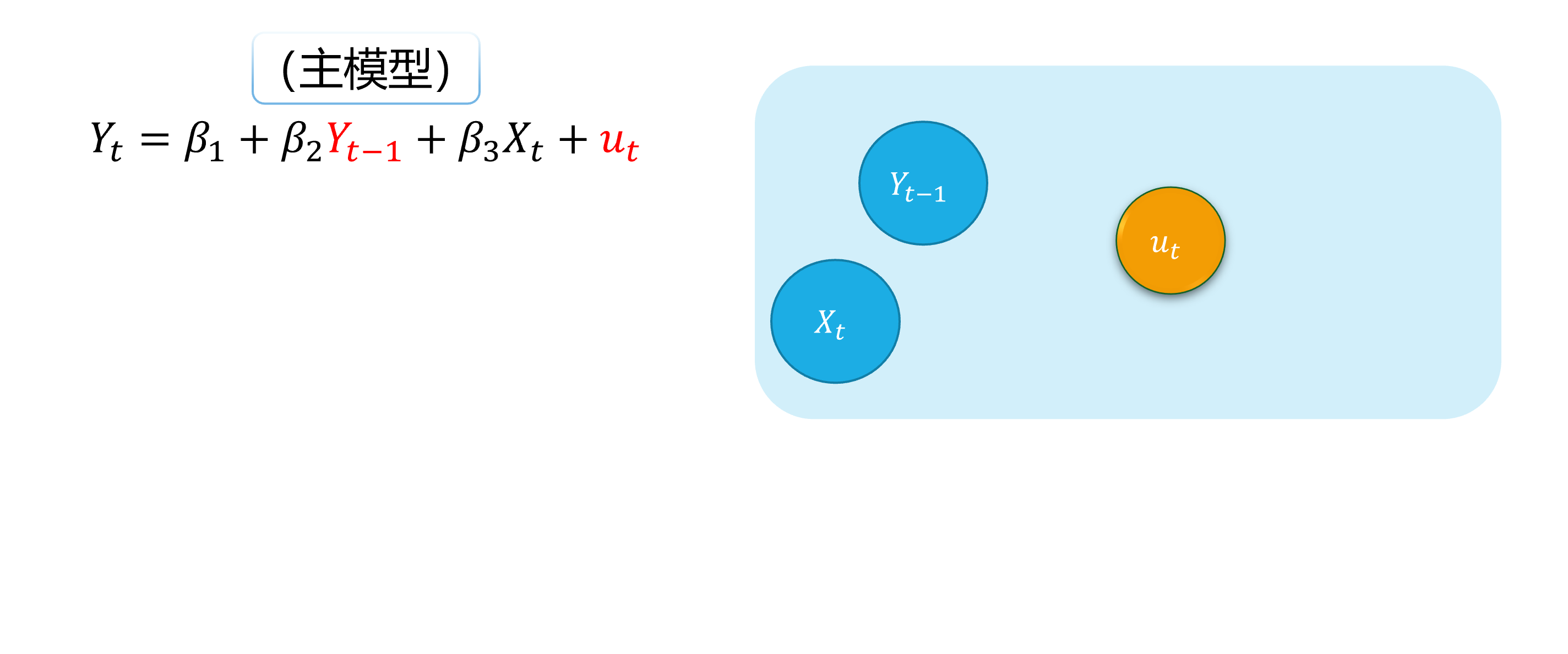：  --- ### 内生自变量情形3：序列自相关（演示2） 具体地，序列自相关引发内生自变量问题的直观演示如下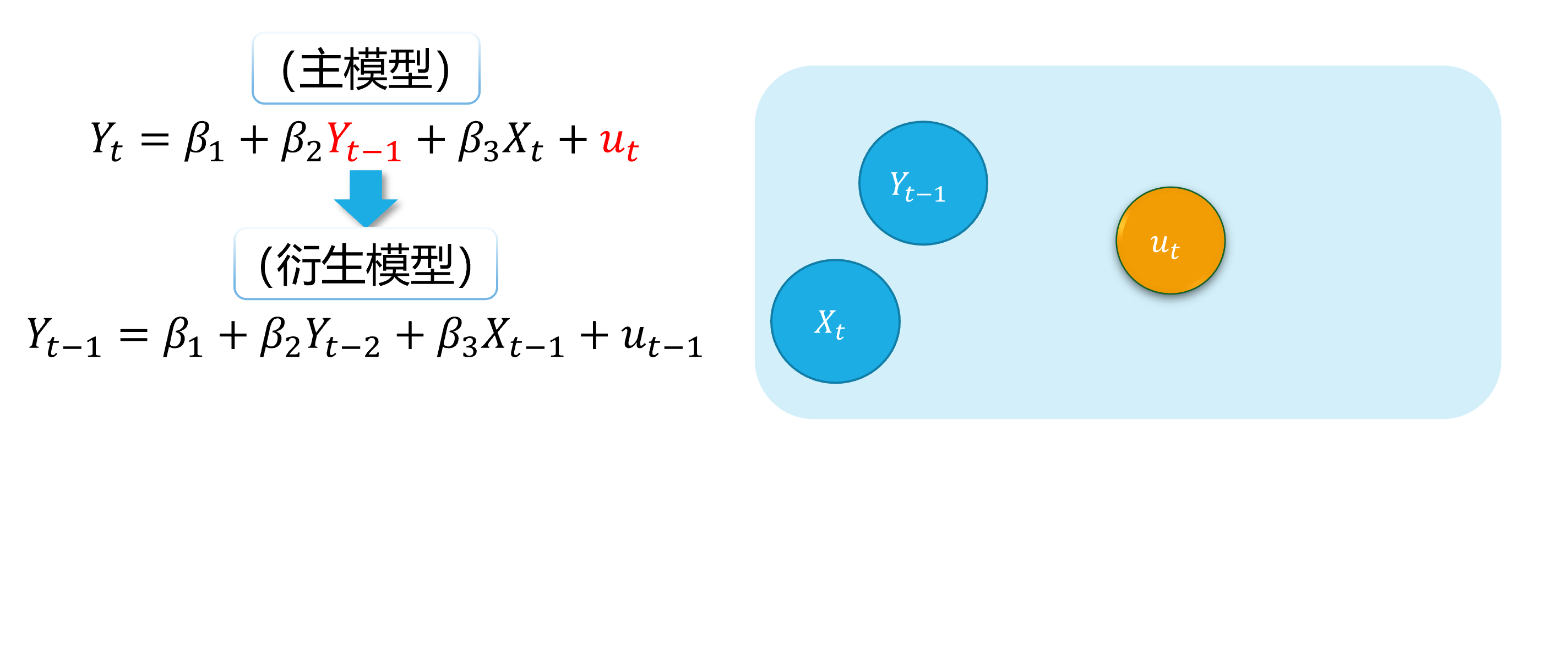：  --- ### 内生自变量情形3：序列自相关（演示2） 具体地，序列自相关引发内生自变量问题的直观演示如下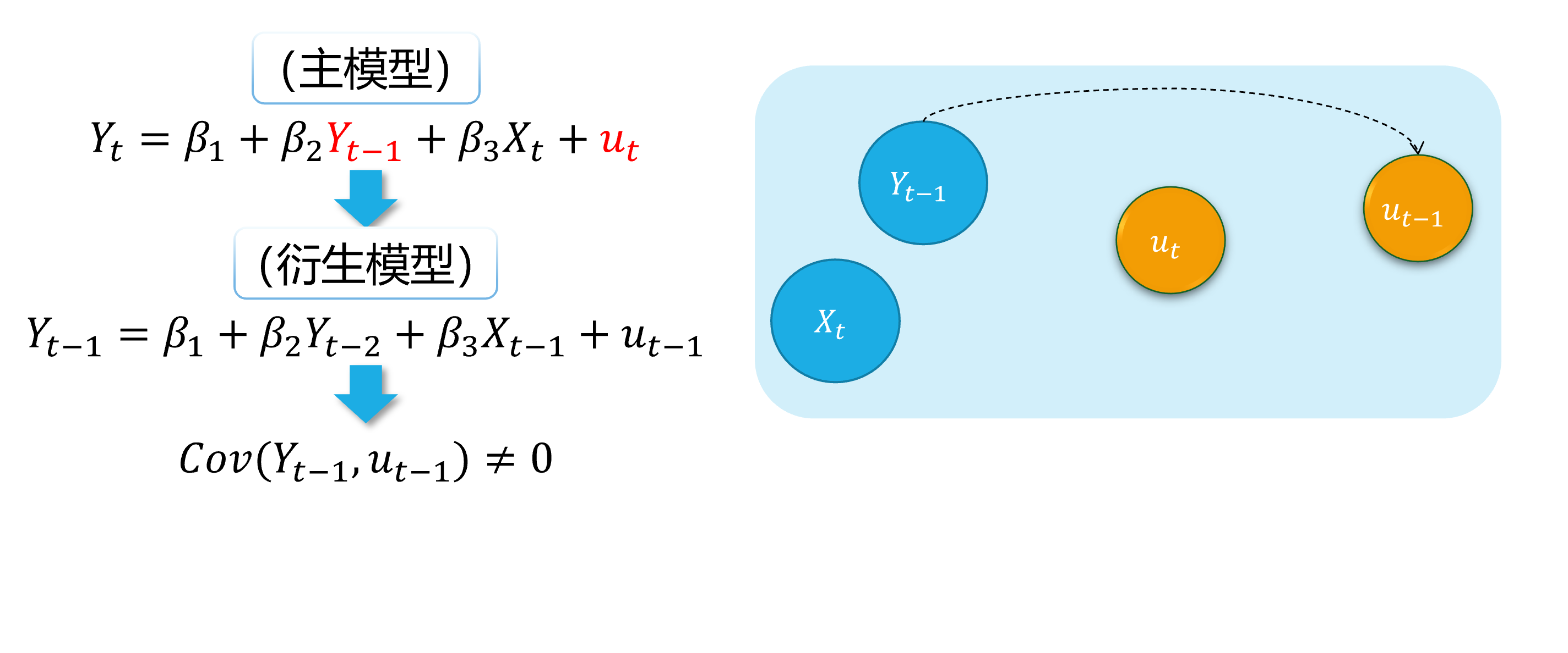：  --- ### 内生自变量情形3：序列自相关（演示2） 具体地，序列自相关引发内生自变量问题的直观演示如下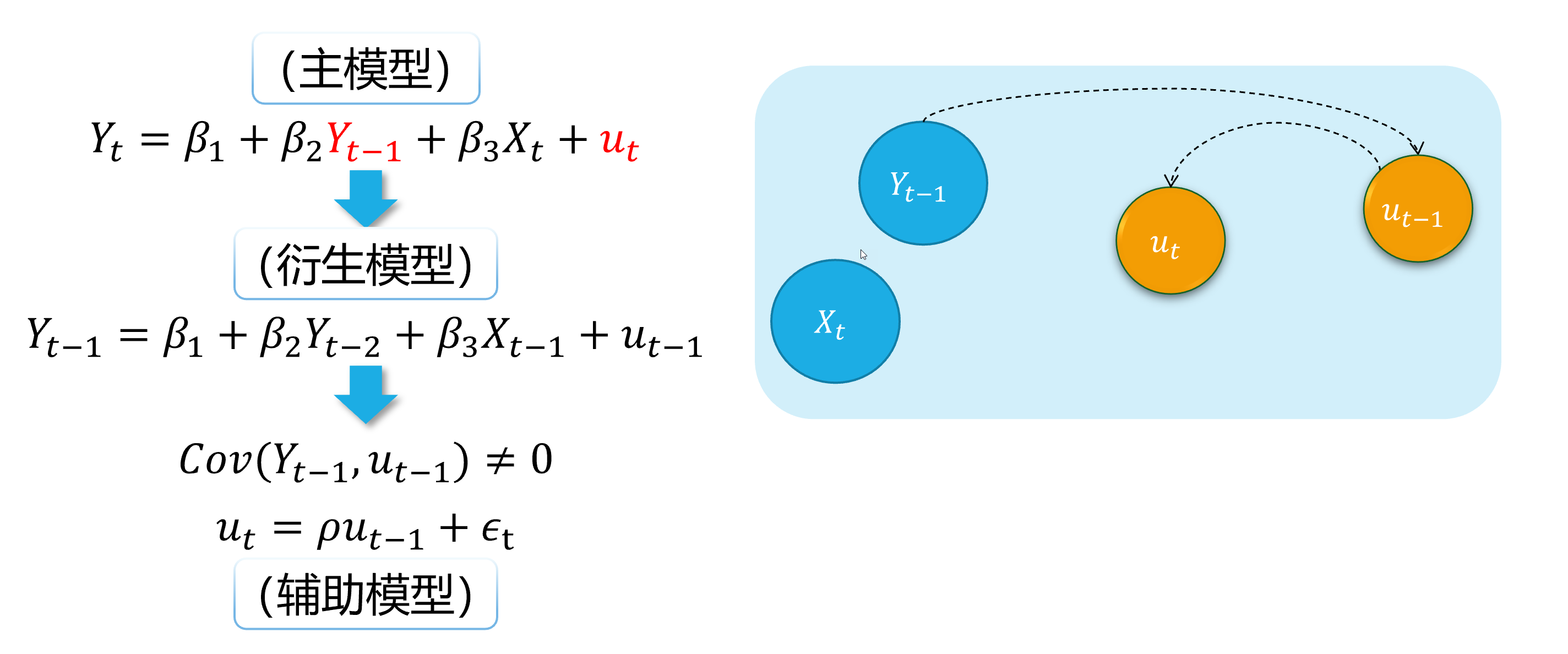：  --- ### 内生自变量情形3：序列自相关（演示2） 具体地，序列自相关引发内生自变量问题的直观演示如下：  --- ### 内生自变量情形4：方程联立性 对于供需联立方程的结构化形式： `$$\begin{cases} \begin{align} \text { Demand: } & Q_{i}=\alpha_{1}+\alpha_{2} P_{i}+u_{d i} \\ \text { Supply: } & Q_{i}=\beta_{1}+\beta_{2} P_{i} + u_{s i} \end{align} \end{cases}$$` 众所周知，因为价格 `\(P_i\)`变动会影响供给量和需求量 `\(Q_i\)`的变动；反之亦然。两者之间存在相互反馈影响机制。 因此，可以证明 `\(cov(P_i, u_{di}) \neq 0\)`，而且 `\(cov(P_i, u_{si}) \neq 0\)`，从而产生内生性问题。 --- --- <!---demo1 sem endo begin---> ### 内生自变量情形4：方程联立性（演示1） 下面我们对方程联立性情形做一个整体的直观演示：  --- ### 内生自变量情形4：方程联立性（演示1） 下面我们对方程联立性情形做一个整体的直观演示：  --- ### 内生自变量情形4：方程联立性（演示1） 下面我们对方程联立性情形做一个整体的直观演示：  --- ### 内生自变量情形4：方程联立性（演示1） 下面我们对方程联立性情形做一个整体的直观演示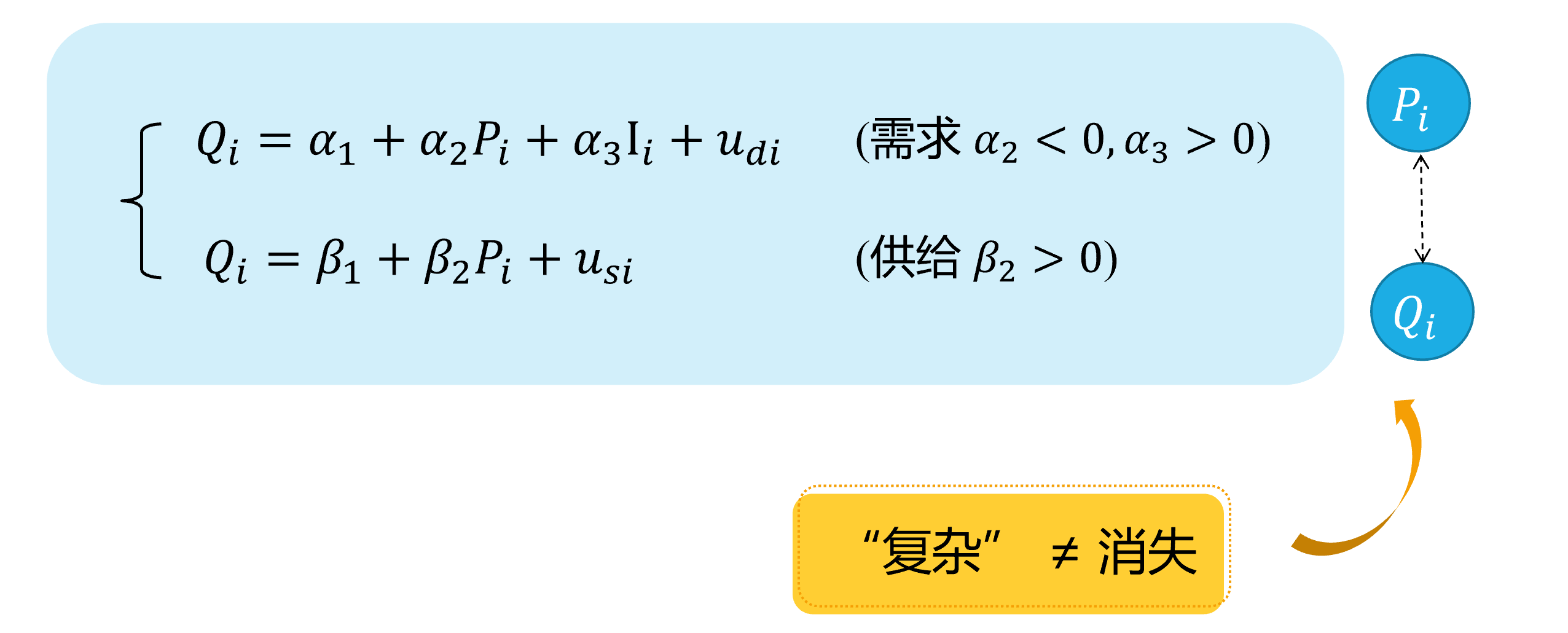：  --- <!---demo2 ar endo begion---> ### 内生自变量情形4：方程联立性（演示2） 具体地，方程联立性引发内生自变量问题的直观演示如下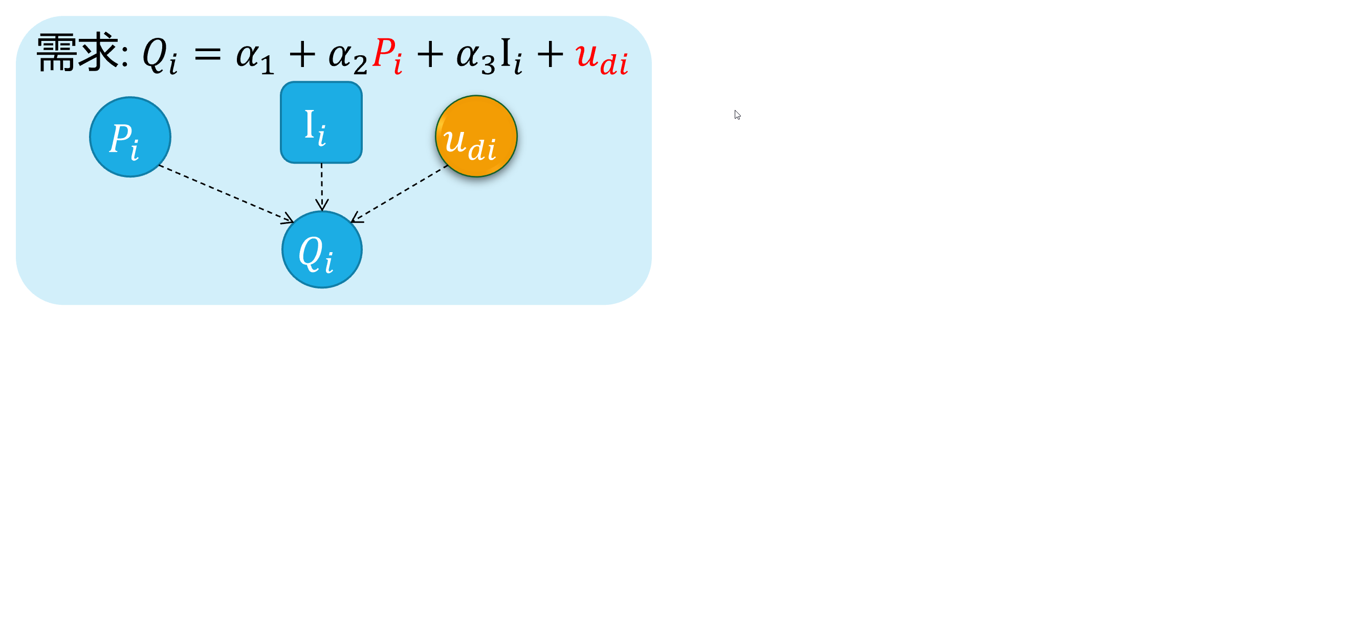：  --- ### 内生自变量情形4：方程联立性（演示2） 具体地，方程联立性引发内生自变量问题的直观演示如下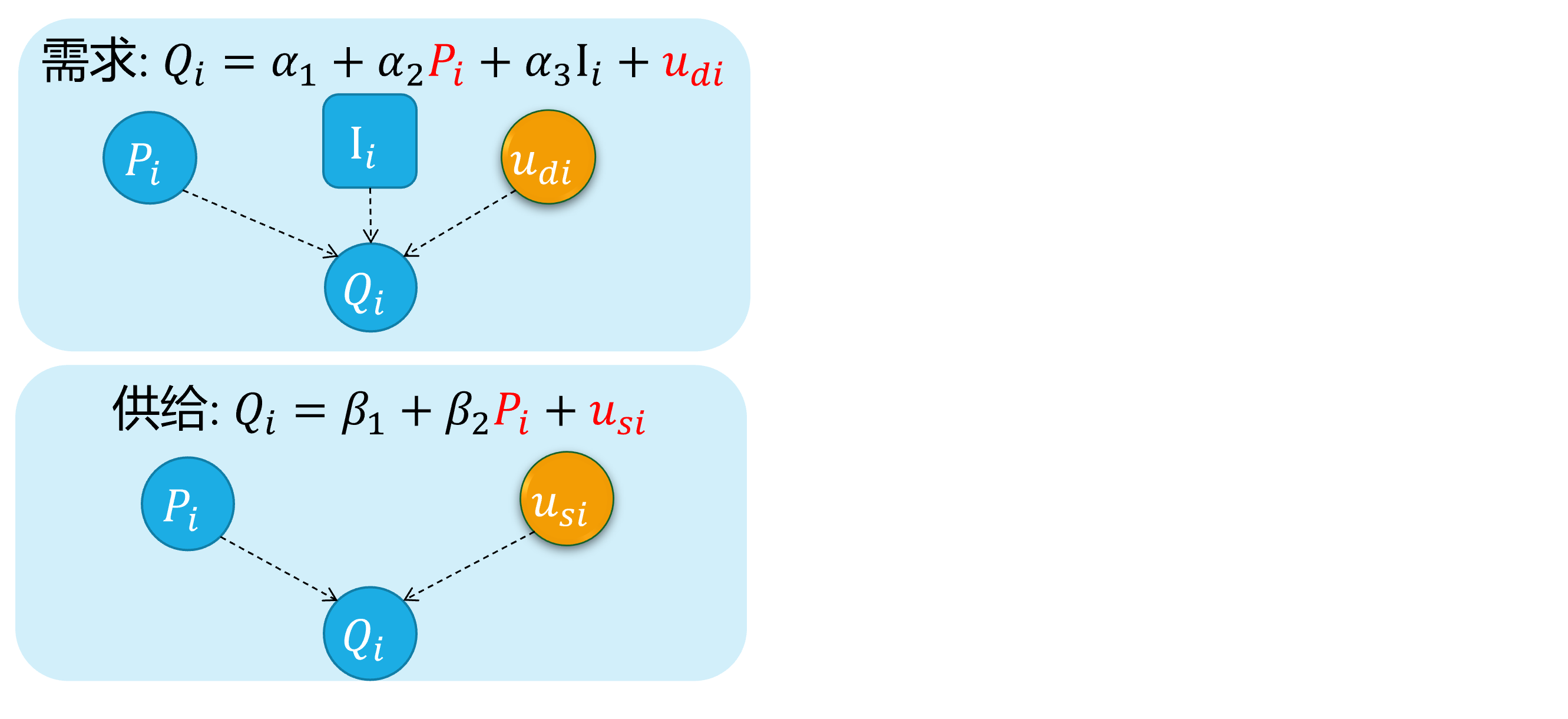：  --- ### 内生自变量情形4：方程联立性（演示2） 具体地，方程联立性引发内生自变量问题的直观演示如下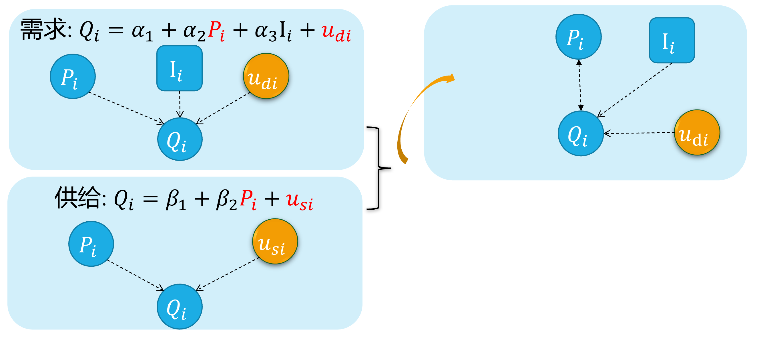：  --- ### 内生自变量情形4：方程联立性（演示2） 具体地，方程联立性引发内生自变量问题的直观演示如下：  --- ### 内生自变量情形4：方程联立性（演示2） 具体地，方程联立性引发内生自变量问题的直观演示如下：  --- ## 学习成绩与逃课次数的例子 假设**“真实模型”**是： `$$\begin {align} score_i=\alpha_{1}+\alpha_{2}skipped_i+ \alpha_3 abil_i + \alpha_4 mot_i + \alpha_5 income_i +u_i \end {align}$$` 一个遗漏了重要变量的**“偏误模型”**是： `$$\begin {align} score_i=\beta_{1}+\beta_{2}skipped_i+v_i \end {align}$$` - 学习成绩受到逃课次数的影响，但是我们也很担心以上模型中 `\(skipped_i\)`与 `\(v_i\)`中的某些因素相关，例如越有能力 `\(abil_i\)`、越积极 `\(mot_i\)`的学生，逃课也越少。 - 因为自变量 `\(skipped_i\)`可能与随机干扰项 `\(v_i\)`相关。此时，对于以上简单的回归，可能得不出可靠的估计。 --- ## 学习成绩与逃课次数的例子 `$$\begin {align} score_i=\beta_{1}+\beta_{2}skipped_i+v_i \end {align}$$` 逃课次数 `\(skipped_i\)`的工具变量 `\(Z_i\)`有哪些可供备选的呢？ -- - 宿舍跟上课地点的距离 `\(distance\)`。我们一般认为，它与逃课次数相关 `\(skipped_i\)`，但是它与 `\(v_i\)`中的某些因素也会相关么？ -- - 如果收入水平 `\(income\)`确实影响了学习成绩，但是模型却没有引入收入水平 `\(income\)`变量，也就意味着 `\(v_i\)`中包含了遗漏的重要变量——收入水平 `\(income\)`。此时，距离 `\(distance\)`就会与收入水平 `\(income\)`相关，进而与 `\(v_i\)`相关。——因为收入少的学生，更倾向于在外租房（合租）；收入多的学生，更倾向于住校。 ??? - 此外，如果能找到能力 `\(abil_i\)`的一个合适的工具变量 `\(Z_{2i}\)`，那么也可以减弱我们对一元回归模型估计问题的担忧。例如，累计学积分 `\(GPA\)`。 --- layout:false class: center, middle, duke-softblue,hide_logo name: problem # 3.4.2 内生变量法下的估计问题 --- layout: true <div class="my-header-h2"></div> <div class="watermark1"></div> <div class="watermark2"></div> <div class="watermark3"></div> <div class="my-footer"><span>huhuaping@ <a href="#chapter-navi">模块01 计量经济学基础 |</a> &emsp;&emsp;&emsp;&emsp; <a href="#chapter03">第03章 放宽假设 |</a> &emsp;&emsp;&emsp;&emsp; <a href="#endogeneity"> 3.4 内生性自变量（endogeneity-variable）问题 |</a> &emsp;&emsp;&emsp;&emsp; <a href="#problem"> 3.4.2 内生变量法下的估计问题 </a> </span></div> --- ## 造成不一致性估计：遗漏变量情形 一般而言，由于A2不成立，相关重要变量的**遗漏**，会导致OLS方法的估计**不一致**。 .pull-left[ 假设真实的**工资**模型是**教育**和**能力**的函数： `$$\begin{align} Wage_{i}=\beta_{1}+\beta_{2} Edu_{i}+\beta_{3} Abl_{i}+u_{i} \quad \text{(a)} \end{align}$$` > 然而个人能力往往是不能被观察到的。 ] .pull-right[ 因此能力被包含在误设模型的**随机干扰项**中: `$$\begin{align} Wage_{i}=\beta_{1}+\beta_{2} Edu_{i}+e_{i} \quad \text{(b)} \end{align}$$` > 其中： `\(e_{i}=\beta_{3} Abl_{i}+\epsilon_{i}\)` ] 问题是能力不仅影响工资，而且能力越强的人受教育的时间越长，这就导致了随机误差项和教育变量之间的正相关。 `\(\operatorname{Cov}\left(Edu_{i}, e_{i}\right)>0\)`. > 牢记: - 遗漏并不等于消失！"omission" does not means “disappear” ! --- ## 造成不一致性估计：测量误差情形 如果**真实模型**为： `$$\begin{align} Y_{i}=\beta_{0}+\beta_{1} X_{i}+\epsilon_{i} \quad \text{(1)} \end{align}$$` 我们希望观测自变量 `\(X\)`对因变量 `\(Y\)`的真实影响，但是很可能我们无法完全地观测得到自变量 `\(X\)`，从而退一步采用一个可以观测到的**代理变量**（如 `\(X^{\ast}\)`）。 `$$\begin{align} X^{\ast}_{i}=X_{i} - v_{i} \quad \text{(2)} \end{align}$$` >其中： - 随机变量 `\(v_i\)`的期望为0，方差为 `\(\sigma_{v}^{2}\)` - `\(X_i, \epsilon_i\)` 与 `\(v_i\)`是互为独立的（**pairwise independent**）。 从而，我们构造了一个包含**测量误差**的**误设模型**： `$$\begin{align} Y_{i}=\alpha_{0}+\alpha_{1} X^{\ast}_{i}+v_{i} \quad \text{(3)} \end{align}$$` --- ## 造成不一致性估计：测量误差情形 更一般地： `$$\begin{align} Y_{i} &=\beta_{0}+\beta_{1} X_{i}+\epsilon_{i} && \text{ eq(1) assumed true model } \end{align}$$` `$$\begin{align} X^{\ast}_i &= X_i - v_i && \text{ eq(2) proxy variable }\\ X_i &= X^{\ast}_i + v_i && \text{ eq(3)}\\ Y_{i} &=\beta_{0}+\beta_{1} X^{\ast}_{i}+u_{i} && \text{ eq(4) error specified model} \end{align}$$` 把方程 (3) 带入方程 (1)，可以得到方程(5)： `$$\begin{align} Y_{i} =\beta_{0}+\beta_{1} X_{i}^{*}+\epsilon_{i} =\beta_{0}+\beta_{1}\left(X^{\ast}_{i} + v_{i}\right)+\epsilon_{i} =\beta_{0}+\beta_{1} X^{\ast}_{i}+\left(\epsilon_{i} + \beta_{1} v_{i}\right) \quad \text{eq(5)} \end{align}$$` 这将表明**误设模型**中的随机误差项 `\(u_{i}=\left(\epsilon_{i}+\beta_{1} v_{i}\right)\)`，从而导致 `\(\operatorname{Cov}\left(X^{\ast}_{i}, u_{i}\right) \neq 0\)`，根据高斯马尔可夫定量，OLS方法将不能得到一致性估计量（具体见下一页）。 --- ## 造成不一致性估计：测量误差情形 容易证明： `\(E\left(u_{i}\right)=E\left(\epsilon_{i} +\beta_{1} v_{i}\right)=E\left(\epsilon_{i}\right)+\beta_{1} E\left(v_{i}\right)=0\)` 然而： `$$\begin{aligned} \operatorname{Cov}\left(X^{\ast}_{i}, u_{i}\right) &=E\left[\left(X^{\ast}_{i}-E\left(X^{\ast}_{i}\right)\right)\left(u_{i}-E\left(u_{i}\right)\right)\right] \\ &=E\left(X^{\ast}_{i} u_{i}\right) \\ &=E\left[\left(X_{i}-v_{i}\right)\left(\epsilon_{i} +\beta_{1} v_{i}\right)\right] \\ &=E\left[X_{i} \epsilon_{i}+\beta_{1} X_{i} v_{i}- v_{i}\epsilon_{i}- \beta_{1} v_{i}^{2}\right] \leftarrow \quad \text{(pairwise independent)} \\ &=-E\left(\beta_{1} v_{i}^{2}\right) \\ &=-\beta_{1} \operatorname{Var}\left(v_{i}\right) \\ &=-\beta_{1} \sigma_{v_i}^{2} \neq 0 \end{aligned}$$` 因此，方程4中的自变量 `\(X^{\ast}\)` 是内生自变量（.red[**endogenous**]），从而OLS的系数估计量 `\(\beta_{1}\)`是不一致的。 ??? So far as we know, both omitted variable(s) and error measurement will cause endogeneity, and result in violation of A2. Let us sum up all these cases in general. --- ## OLS估计: 违背CLRM假设A2 一般而言, 如果CLRM假设中的**A2**被违背，OLS估计量将会是**有偏的**（biased estimator）: 我们已知，真实参数 `\(\hat{\beta}\)`的OLS估计量理论公式为： `$$\begin{align} \widehat{\beta} &=\beta+\left(X^{\prime} X\right)^{-1} X^{\prime} \epsilon && \text{(6)} \end{align}$$` 我们可以两边同时取期望： `$$\begin{equation} \begin{aligned} E(\widehat{\beta}) &=\beta+E\left(\left(X^{\prime} X\right)^{-1} X^{\prime} \epsilon\right) \\ &=\beta+E\left(E\left(\left(X^{\prime} X\right)^{-1} X^{\prime} \epsilon | X\right)\right) \\ &=\beta+E\left(\left(X^{\prime} X\right)^{-1} X^{\prime} E(\epsilon | X)\right) \neq \beta \end{aligned} \end{equation}$$` 如果CLRM假设中**A2** `\(E(\epsilon | X) = 0\)`被违背，也即意味着 `\(E(\epsilon | X) \neq 0\)`，从而OLS估计量是有偏的。 --- ## OLS估计: 一致性估计量 那么，在什么条件下我们才能得到一致估计量呢？ `$$\begin{equation} \begin{aligned} p \lim \widehat{\beta} &=\beta+p \lim \left(\left(X^{\prime} X\right)^{-1} X^{\prime} \epsilon\right) =\beta+p \lim \left(\left(\frac{1}{n} X^{\prime} X\right)^{-1} \frac{1}{n} X^{\prime} \epsilon\right) \\ &=\beta+p \lim \left(\frac{1}{n} X^{\prime} X\right)^{-1} \times p \lim \left(\frac{1}{n} X^{\prime} \epsilon\right) \end{aligned} \end{equation}$$` 通过**弱大数定律**(Weak Law of Large Numbers, WLLN)： `$$\begin{equation} \frac{1}{n} X^{\prime} \epsilon=\frac{1}{n} \sum_{i=1}^{n} X_{i} \epsilon_{i} \xrightarrow{p} E\left(X_{i} \epsilon_{i}\right) \end{equation}$$` 因此如果 `\(E\left(X_{i} \epsilon_{i}\right)=0\)`，则 `\(\widehat{\beta}\)`是一致估计量。 > 需要注意的是： `\(E\left(X_{i} \epsilon_{i}\right)=0\)` 比CLRM假设中的A2 `\(E(\epsilon | X) = 0\)`更容易满足。因此，一些**有偏**的估计量，在大样本情况下也可以是**渐进一致的**。 --- ## 工资案例：误设模型 考虑如下的“误设模型”: `$$\begin{align} lwage_i = \beta_1 +\beta_2educ_i + \beta_3exper_i +\beta_4expersq_i + v_i \end{align}$$` 如前所述，该“误设模型”的问题在于，随机误差项中包含不可观测的重要变量，例如个人**能力水平**（ `\(Abl_i\)`）, 它同时对**工资水平**因变量和**受教育程度**自变量产生影响。 换言之，自变量**工资水平**与随机干扰项相关，也即 `\(cov(educ_i, v_i) \neq 0\)`，因此它是内生自变量（endogenous regressor）。 > **注意**： - 在实践中，我们将使用**受教育年数**作为**educ**的代理变量，这本身也会带来前面提到的**误差测量**问题。 --- ## 案例变量说明 研究者关注428名已婚女性**时均工资** `\(wage\)`与其**受教育年数** `\(educ\)`之间的关系，并考虑如下变量： <div id="htmlwidget-2365ab4815dc44fbe47a" style="width:100%;height:auto;" class="datatables html-widget"></div> <script type="application/json" data-for="htmlwidget-2365ab4815dc44fbe47a">{"x":{"filter":"none","caption":"<caption>变量说明<\/caption>","data":[["1","2","3","4","5","6","7","8","9","10","11","12","13","14","15","16","17","18","19","20","21","22"],["lwage","educ","exper","fatheduc","motheduc","inlf","hours","kidslt6","kidsge6","age","wage","repwage","hushrs","husage","huseduc","huswage","faminc","mtr","unem","city","nwifeinc","expersq"],["时均工资","受教育年数","就业次数","父亲的受教育年数","母亲的受教育年数","是否是劳动力","工作时长","六岁以下孩子数","6-18岁孩子数","年龄","回访年的时均工资","丈夫工作时长","丈夫年龄","丈夫的受教育年数","丈夫的时均工资","家庭收入","征收税率","所在地区失业率","居住地是否为SMSA","扣除妇女工资的家庭收入/1000","工资的对数","就业次数的平方"]],"container":"<table class=\"display\">\n <thead>\n <tr>\n <th> <\/th>\n <th>vars<\/th>\n <th>mark<\/th>\n <\/tr>\n <\/thead>\n<\/table>","options":{"dom":"tip","columnDefs":[{"className":"dt-center","targets":"_all"},{"visible":false,"targets":0},{"orderable":false,"targets":0}],"pageLength":7,"order":[],"autoWidth":false,"orderClasses":false,"lengthMenu":[7,10,25,50,100]}},"evals":[],"jsHooks":[]}</script> --- ## 案例原始数据 <div id="htmlwidget-d932baf20ee00ee0133e" style="width:100%;height:auto;" class="datatables html-widget"></div> <script type="application/json" data-for="htmlwidget-d932baf20ee00ee0133e">{"x":{"filter":"none","caption":"<caption>数据集 （n=428）<\/caption>","data":[["1","2","3","4","5","6","7","8","9","10","11","12","13","14","15","16","17","18","19","20","21","22","23","24","25","26","27","28","29","30","31","32","33","34","35","36","37","38","39","40","41","42","43","44","45","46","47","48","49","50","51","52","53","54","55","56","57","58","59","60","61","62","63","64","65","66","67","68","69","70","71","72","73","74","75","76","77","78","79","80","81","82","83","84","85","86","87","88","89","90","91","92","93","94","95","96","97","98","99","100","101","102","103","104","105","106","107","108","109","110","111","112","113","114","115","116","117","118","119","120","121","122","123","124","125","126","127","128","129","130","131","132","133","134","135","136","137","138","139","140","141","142","143","144","145","146","147","148","149","150","151","152","153","154","155","156","157","158","159","160","161","162","163","164","165","166","167","168","169","170","171","172","173","174","175","176","177","178","179","180","181","182","183","184","185","186","187","188","189","190","191","192","193","194","195","196","197","198","199","200","201","202","203","204","205","206","207","208","209","210","211","212","213","214","215","216","217","218","219","220","221","222","223","224","225","226","227","228","229","230","231","232","233","234","235","236","237","238","239","240","241","242","243","244","245","246","247","248","249","250","251","252","253","254","255","256","257","258","259","260","261","262","263","264","265","266","267","268","269","270","271","272","273","274","275","276","277","278","279","280","281","282","283","284","285","286","287","288","289","290","291","292","293","294","295","296","297","298","299","300","301","302","303","304","305","306","307","308","309","310","311","312","313","314","315","316","317","318","319","320","321","322","323","324","325","326","327","328","329","330","331","332","333","334","335","336","337","338","339","340","341","342","343","344","345","346","347","348","349","350","351","352","353","354","355","356","357","358","359","360","361","362","363","364","365","366","367","368","369","370","371","372","373","374","375","376","377","378","379","380","381","382","383","384","385","386","387","388","389","390","391","392","393","394","395","396","397","398","399","400","401","402","403","404","405","406","407","408","409","410","411","412","413","414","415","416","417","418","419","420","421","422","423","424","425","426","427","428"],[1,2,3,4,5,6,7,8,9,10,11,12,13,14,15,16,17,18,19,20,21,22,23,24,25,26,27,28,29,30,31,32,33,34,35,36,37,38,39,40,41,42,43,44,45,46,47,48,49,50,51,52,53,54,55,56,57,58,59,60,61,62,63,64,65,66,67,68,69,70,71,72,73,74,75,76,77,78,79,80,81,82,83,84,85,86,87,88,89,90,91,92,93,94,95,96,97,98,99,100,101,102,103,104,105,106,107,108,109,110,111,112,113,114,115,116,117,118,119,120,121,122,123,124,125,126,127,128,129,130,131,132,133,134,135,136,137,138,139,140,141,142,143,144,145,146,147,148,149,150,151,152,153,154,155,156,157,158,159,160,161,162,163,164,165,166,167,168,169,170,171,172,173,174,175,176,177,178,179,180,181,182,183,184,185,186,187,188,189,190,191,192,193,194,195,196,197,198,199,200,201,202,203,204,205,206,207,208,209,210,211,212,213,214,215,216,217,218,219,220,221,222,223,224,225,226,227,228,229,230,231,232,233,234,235,236,237,238,239,240,241,242,243,244,245,246,247,248,249,250,251,252,253,254,255,256,257,258,259,260,261,262,263,264,265,266,267,268,269,270,271,272,273,274,275,276,277,278,279,280,281,282,283,284,285,286,287,288,289,290,291,292,293,294,295,296,297,298,299,300,301,302,303,304,305,306,307,308,309,310,311,312,313,314,315,316,317,318,319,320,321,322,323,324,325,326,327,328,329,330,331,332,333,334,335,336,337,338,339,340,341,342,343,344,345,346,347,348,349,350,351,352,353,354,355,356,357,358,359,360,361,362,363,364,365,366,367,368,369,370,371,372,373,374,375,376,377,378,379,380,381,382,383,384,385,386,387,388,389,390,391,392,393,394,395,396,397,398,399,400,401,402,403,404,405,406,407,408,409,410,411,412,413,414,415,416,417,418,419,420,421,422,423,424,425,426,427,428],[1.2101536989212,0.328512102365494,1.51413774490356,0.0921233221888542,1.52427220344543,1.55648005008698,2.12025952339172,2.0596342086792,0.754336357116699,1.54489934444427,1.4019216299057,1.52427220344543,0.733953237533569,0.818369090557098,1.30283117294312,0.298028379678726,1.16760957241058,1.64383935928345,0.6931471824646,2.02193164825439,1.25424754619598,1.27295768260956,1.1786550283432,1.1786550283432,0.767558693885803,1.33181178569794,1.3862943649292,1.55326962471008,1.98181486129761,1.76936042308807,0.430807888507843,0.899754822254181,1.76662969589233,1.27295768260956,1.33678889274597,0.901704847812653,0.865123689174652,1.51184713840485,1.72602915763855,2.68314242362976,0.985294282436371,1.36593854427338,0.945033669471741,1.51237618923187,0.6931471824646,1.24478840827942,0.701164901256561,1.5198632478714,0.820968568325043,0.969831526279449,0.828508198261261,0.0943096429109573,0.162543892860413,0.470003634691238,0.629248440265656,1.39716017246246,2.26544380187988,2.0845410823822,1.52583885192871,0.762160062789917,1.48160457611084,1.26282644271851,0.999675571918488,1.83258152008057,2.47930765151978,1.27901530265808,1.93793559074402,1.0704528093338,1.12392258644104,1.32175588607788,1.74499976634979,1.30174362659454,1.64186644554138,2.10702013969421,1.46706759929657,1.60581135749817,-1.02973937988281,1.08768618106842,0,0.938208699226379,-0.150590375065804,0,1.07367050647736,1.26584839820862,0.486368983983994,2.12025952339172,1.12985253334045,0.993251800537109,1.65862798690796,0.347412198781967,1.56832420825958,0.510845601558685,0.114845432341099,-0.6931471824646,-0.336452275514603,1.02822554111481,1.58068859577179,0.555894613265991,0.901420712471008,0.884304583072662,0.428204596042633,1.05841505527496,0.87833958864212,1.65490829944611,1.32175588607788,0.328512102365494,1.3862943649292,1.17288458347321,1.22418713569641,0.287657082080841,2.23026180267334,1.50407743453979,1.53115200996399,1.37515759468079,1.76026880741119,-0.6931471824646,1.40648913383484,1.7917594909668,1.29929208755493,1.35100388526917,1.01628088951111,1.0753436088562,1.47896468639374,1.68948674201965,2.28859782218933,-1.82263112068176,-0.960765182971954,1.29099416732788,0.864871144294739,1.54045212268829,0.616212129592896,1.64865863323212,1.19349813461304,2.14397621154785,0.724403560161591,0.941607534885406,0.782759368419647,1.83258152008057,1.20396280288696,1.49164485931396,1.89213263988495,2.13089489936829,1.48060405254364,0.894331336021423,0.202532544732094,0.485507816076279,1.0986123085022,1.55326962471008,0.121597968041897,2.00180435180664,1.49503660202026,0.905229806900024,0.632547557353973,1.3862943649292,2.10291385650635,1.95964395999908,0.510845601558685,1.23692393302917,1.44331252574921,1.02165925502777,0.63615345954895,1.61645328998566,0.223143547773361,1.04980707168579,1.41505193710327,0.575376629829407,2.60668158531189,1.51791453361511,0.755041599273682,1.09497237205505,0.942114353179932,1.72494280338287,1.03154611587524,0.474369078874588,0.810930192470551,0.709266602993011,1.71054947376251,0.460268884897232,1.33181178569794,1.0986123085022,2.15799856185913,1.43758130073547,1.54489934444427,1.41059672832489,3.21887588500977,0.968161880970001,1.7917594909668,1.68872952461243,-0.409171968698502,0.223143547773361,0.822155833244324,1.24170196056366,1.42712438106537,1.49709749221802,0.559615790843964,1.30002820491791,1.88442981243134,0.955511391162872,1.58208727836609,1.7556140422821,1.51310324668884,2.25189161300659,2.3644323348999,0.105350479483604,1.39972877502441,0.988462507724762,1.09064733982086,1.15461444854736,1.26694762706757,2.88519167900085,1.22888004779816,1.20396280288696,1.35738027095795,0.837723612785339,0.536961138248444,0.748723804950714,2.29587268829346,1.10780322551727,0.620845258235931,-2.05416369438171,1.89201200008392,1.72972452640533,0.469378411769867,0.98084169626236,2.06949234008789,1.67518818378448,1.3862943649292,1.79921495914459,1.83258152008057,1.09064733982086,1.44312357902527,1.25036013126373,1.60231256484985,1.01855850219727,1.29705321788788,1.68519449234009,-0.420984894037247,1.56209468841553,2.14652752876282,2.34746289253235,0.969831526279449,1.9241464138031,1.62672758102417,-0.0392607264220715,1.46014869213104,1.95539355278015,0.926359891891479,2.06619167327881,1.42284321784973,2.10103178024292,2.26146101951599,0.70131379365921,2.03101253509521,1.16236925125122,0.470003634691238,1.41059672832489,0.393055111169815,1.29099416732788,0,0.95712548494339,0.559615790843964,1.56861591339111,1.7101879119873,1.41059672832489,0.223143547773361,0.510845601558685,1.33239245414734,0.860185861587524,2.32277989387512,1.91959547996521,1.97610676288605,0.895434737205505,0.18123759329319,0.495305836200714,0.577792406082153,1.07881772518158,1.60319852828979,0.620845258235931,2.08389401435852,1.37916910648346,1.11238372325897,1.06712162494659,1.11880695819855,1.58854103088379,1.3903112411499,1.71480643749237,0.20106153190136,0.987271010875702,0.98350065946579,2.23317074775696,1.14361751079559,-0.611382901668549,2.15305209159851,1.29983735084534,0.840920448303223,1.05848443508148,1.15265846252441,1.29357588291168,1.83258152008057,2.32718014717102,1.16614627838135,2.03499317169189,0.679251074790955,1.54713690280914,0.75301855802536,0.847283601760864,0.871125996112823,0.228250473737717,0.0896578282117844,1.32175588607788,1.19610190391541,1.63611876964569,1.89201200008392,1.51830899715424,2.47215914726257,1.32175588607788,1.47364103794098,1.36947882175446,1.20396280288696,1.19872915744781,1.27020990848541,0.470003634691238,0.799981653690338,1.56594562530518,1.75897800922394,0.858025848865509,0.6931471824646,0.641853868961334,1.63374018669128,1.70374763011932,1.84400403499603,1.96611881256104,0.864997446537018,0.933305203914642,0.779233157634735,0.955511391162872,1.31624734401703,1.4759064912796,1.49139726161957,1.45575046539307,0.510845601558685,1.18043804168701,1.68848943710327,0.790727496147156,1.40179860591888,-0.433556020259857,1.68317151069641,-1.76667666435242,3.15559506416321,2.25952100753784,1.30692636966705,0.798497676849365,0.559044182300568,0.147902622818947,1.94449484348297,1.37833786010742,3.0647451877594,-0.741917312145233,0.765700399875641,0.619392991065979,1.46545207500458,2.18925952911377,1.02165925502777,0.977009475231171,0.916290760040283,2.90509605407715,-0.199671193957329,0.6931471824646,2.73339295387268,1.86833465099335,2.12025952339172,1.51519322395325,0.914609313011169,1.49955606460571,0.803077220916748,0.728031635284424,0.516409993171692,1.22644829750061,0.916290760040283,1.37647128105164,1.8289749622345,1.36828315258026,1.06471073627472,1.40648913383484,1.04731893539429,1.94809341430664,1.07800137996674,0.653938472270966,1.92789161205292,1.36102783679962,0.6931471824646,1.60468661785126,0.183903649449348,3.11351537704468,1.92682921886444,1.2701256275177,0.68269270658493,1.68106997013092,0.556295990943909,1.62822043895721,0.916290760040283,1.3415584564209,0,1.12223124504089,0.540170788764954,1.3915057182312,1.69717395305634,3.21887588500977,0.871167778968811,1.16732954978943,1.21698772907257,0.575376629829407,1.15161573886871,0.994251251220703,0.526324927806854,-1.5431821346283,1.91204309463501,0.554287314414978,0.916290760040283,1.50093913078308,0.944683790206909,1.24126863479614,1.56498432159424,0.838026463985443,1.66885709762573,1.7694286108017,1.22644829750061,1.40648913383484],[12,12,12,12,14,12,16,12,12,12,12,11,12,12,10,11,12,12,12,12,16,12,13,12,12,17,12,12,17,12,11,16,13,12,16,11,12,10,14,17,12,12,16,12,12,12,16,12,12,12,12,12,12,8,10,16,14,17,14,12,14,12,8,12,12,8,17,12,12,12,12,12,9,10,12,12,12,17,15,12,6,14,12,14,9,17,13,9,15,12,12,12,12,12,12,12,12,13,12,13,12,12,12,16,12,13,11,12,12,12,17,14,16,17,12,11,12,12,17,10,13,11,12,16,17,12,16,12,16,8,12,12,12,13,11,12,12,14,12,12,12,17,14,12,9,12,12,12,14,16,17,15,12,16,17,17,12,16,13,12,11,16,14,16,12,9,17,14,12,12,11,12,12,10,12,5,17,11,12,12,14,11,12,14,12,10,16,13,12,12,12,11,12,9,13,12,12,12,13,16,12,16,17,12,12,9,12,12,13,12,12,12,12,10,12,16,12,11,12,10,12,12,12,12,16,17,12,17,12,12,12,8,12,13,12,12,8,12,17,17,12,13,12,12,12,12,9,10,12,16,13,8,16,13,12,11,13,12,12,10,12,17,15,16,10,11,12,12,14,16,14,8,7,12,12,14,12,12,12,14,16,12,12,12,13,13,10,12,12,12,12,14,17,10,9,12,12,16,12,17,12,17,11,16,11,13,11,8,11,12,10,17,12,12,17,14,12,12,12,12,12,12,9,10,12,12,12,12,12,17,12,17,12,10,12,12,12,12,12,12,16,13,13,12,16,17,12,14,12,17,12,14,12,12,17,16,16,12,9,12,12,16,14,12,12,11,12,16,17,17,14,12,14,12,10,12,13,16,12,7,16,14,12,10,12,16,10,12,14,12,6,15,12,17,14,13,6,16,14,15,14,8,14,12,12,12,12,12,12,8,12,17,12,12,14,13,17,8,12,11,12,12,17,10,12,13,12,12],[14,5,15,6,7,33,11,35,24,21,15,14,0,14,6,9,20,6,23,9,5,11,18,15,4,21,31,9,7,7,32,11,16,14,27,0,17,28,24,11,1,14,6,10,6,4,10,22,16,6,12,32,15,17,34,9,37,10,35,6,19,10,11,15,12,12,14,11,9,24,12,13,29,11,13,19,2,24,9,6,22,30,10,6,29,29,36,19,8,13,16,11,15,6,13,22,24,2,6,2,2,14,9,11,9,6,19,26,19,3,7,28,13,9,15,20,29,9,1,8,19,23,3,13,8,17,4,15,11,7,0,0,10,8,2,4,6,18,3,22,33,28,23,27,11,6,11,14,17,17,14,11,7,8,6,8,4,25,24,11,19,9,19,14,22,6,23,15,6,11,2,22,10,14,12,9,13,18,8,11,9,9,14,9,2,12,15,11,7,9,19,11,8,13,4,7,19,14,14,3,9,7,7,14,29,19,14,16,10,12,24,6,9,14,26,7,4,15,23,1,29,9,6,11,17,6,7,2,24,4,11,25,11,2,19,7,2,20,10,19,17,12,11,6,10,4,2,13,21,9,4,2,19,4,9,14,6,24,1,13,3,10,16,9,19,4,10,5,7,3,38,16,13,1,7,15,10,2,19,25,25,7,15,11,25,19,4,14,19,18,14,11,4,29,21,24,19,31,28,15,27,13,4,10,8,4,18,3,11,8,10,33,19,35,21,7,18,4,12,16,14,3,1,27,12,6,9,2,6,9,16,22,26,11,11,15,13,6,20,17,8,13,15,14,14,6,24,10,2,9,23,12,8,16,10,7,19,2,9,14,9,16,7,6,22,9,9,14,17,12,13,8,10,16,1,6,4,8,4,15,7,14,16,15,23,19,4,12,12,25,14,14,11,7,18,4,37,13,14,17,5,2,0,3,21,20,19,4,19,11,14,8,13,24,1,1,3,4,21,10,13,9,14,2,21,22,14,7],[196,25,225,36,49,1089,121,1225,576,441,225,196,0,196,36,81,400,36,529,81,25,121,324,225,16,441,961,81,49,49,1024,121,256,196,729,0,289,784,576,121,1,196,36,100,36,16,100,484,256,36,144,1024,225,289,1156,81,1369,100,1225,36,361,100,121,225,144,144,196,121,81,576,144,169,841,121,169,361,4,576,81,36,484,900,100,36,841,841,1296,361,64,169,256,121,225,36,169,484,576,4,36,4,4,196,81,121,81,36,361,676,361,9,49,784,169,81,225,400,841,81,1,64,361,529,9,169,64,289,16,225,121,49,0,0,100,64,4,16,36,324,9,484,1089,784,529,729,121,36,121,196,289,289,196,121,49,64,36,64,16,625,576,121,361,81,361,196,484,36,529,225,36,121,4,484,100,196,144,81,169,324,64,121,81,81,196,81,4,144,225,121,49,81,361,121,64,169,16,49,361,196,196,9,81,49,49,196,841,361,196,256,100,144,576,36,81,196,676,49,16,225,529,1,841,81,36,121,289,36,49,4,576,16,121,625,121,4,361,49,4,400,100,361,289,144,121,36,100,16,4,169,441,81,16,4,361,16,81,196,36,576,1,169,9,100,256,81,361,16,100,25,49,9,1444,256,169,1,49,225,100,4,361,625,625,49,225,121,625,361,16,196,361,324,196,121,16,841,441,576,361,961,784,225,729,169,16,100,64,16,324,9,121,64,100,1089,361,1225,441,49,324,16,144,256,196,9,1,729,144,36,81,4,36,81,256,484,676,121,121,225,169,36,400,289,64,169,225,196,196,36,576,100,4,81,529,144,64,256,100,49,361,4,81,196,81,256,49,36,484,81,81,196,289,144,169,64,100,256,1,36,16,64,16,225,49,196,256,225,529,361,16,144,144,625,196,196,121,49,324,16,1369,169,196,289,25,4,0,9,441,400,361,16,361,121,196,64,169,576,1,1,9,16,441,100,169,81,196,4,441,484,196,49],[7,7,7,7,14,7,7,3,7,7,3,7,16,10,7,10,7,12,7,7,16,10,3,7,7,14,7,7,12,12,7,3,10,14,12,3,3,3,7,17,12,9,16,3,7,7,16,10,7,7,7,3,7,7,3,12,7,17,7,7,3,12,7,7,7,12,16,7,7,7,12,10,9,0,10,14,7,3,12,12,7,17,3,7,7,12,7,7,12,10,0,12,10,7,7,7,3,12,7,12,7,7,10,14,7,12,7,7,10,7,12,7,7,17,7,7,7,10,10,12,7,12,7,10,7,10,7,7,7,7,7,7,16,12,7,3,7,7,7,12,7,12,12,14,7,7,7,12,12,14,10,12,7,16,7,17,3,10,9,7,3,16,12,7,7,7,12,3,7,7,7,7,10,10,7,12,17,10,7,7,12,7,12,7,7,7,7,14,7,12,7,7,12,3,7,12,12,7,7,14,12,17,17,7,7,10,7,7,7,3,0,7,12,7,7,12,7,7,12,7,7,3,7,7,10,12,7,12,7,7,7,7,12,7,7,7,7,7,14,17,7,10,7,7,12,7,7,9,7,14,7,3,16,3,16,7,16,12,7,7,12,12,12,16,7,9,7,12,12,10,7,12,7,7,3,10,17,7,3,3,12,7,7,7,10,7,10,7,9,9,12,12,12,7,9,12,7,12,7,12,12,14,7,14,10,12,7,7,12,7,7,12,12,12,12,14,10,7,7,7,7,7,7,7,7,7,12,12,7,14,10,12,7,7,12,7,10,12,10,7,14,7,12,12,7,16,0,12,7,17,7,12,3,7,14,7,12,12,7,7,14,7,12,12,7,7,7,7,3,12,7,7,14,10,10,10,10,12,3,7,16,7,7,0,7,7,10,7,12,7,7,7,7,16,12,10,7,7,16,7,7,7,12,10,10,10,7,10,12,12,7,17,12,16,10,16,7,7,9,3,7,7,7,7,7,7,16,12],[12,7,12,7,12,14,14,3,7,7,12,14,16,10,7,16,10,12,7,12,10,12,7,7,12,16,3,3,12,12,7,3,12,7,12,10,3,10,7,14,12,9,14,3,12,12,14,10,7,12,7,7,12,7,7,12,7,17,17,12,14,12,7,7,7,12,12,12,7,12,12,10,7,0,7,12,7,3,10,7,12,12,7,7,7,7,7,7,7,10,7,12,10,12,7,7,7,14,7,12,12,7,7,14,12,10,7,7,7,7,12,7,12,10,10,7,7,7,12,7,7,12,14,12,7,10,7,7,12,10,7,7,12,10,7,12,7,7,7,7,3,12,16,7,3,12,7,12,12,16,12,12,7,14,7,10,7,14,7,7,12,12,17,7,7,3,12,7,7,7,3,7,10,10,12,7,14,10,7,7,10,12,12,7,7,7,12,7,12,12,12,10,12,10,12,12,12,7,12,12,12,12,16,7,16,7,7,10,12,10,0,7,12,12,10,12,3,7,12,10,7,7,7,7,12,12,7,12,7,10,10,7,12,17,7,7,7,7,12,14,7,12,7,7,16,7,10,12,7,16,10,3,16,7,12,7,7,7,12,12,7,10,14,16,7,10,7,14,14,12,7,7,3,7,7,7,12,10,7,3,12,7,12,7,10,7,0,7,10,9,12,12,12,3,9,12,12,14,7,12,12,12,7,12,10,12,7,7,3,12,7,16,12,12,7,14,7,7,12,10,7,3,7,7,10,7,7,12,12,12,10,14,7,7,14,10,10,7,7,7,14,7,12,14,14,14,0,16,7,12,7,10,7,10,10,14,7,12,7,7,12,14,12,7,7,7,12,16,3,16,7,16,7,10,10,10,10,12,10,7,16,7,7,7,7,7,10,10,12,7,7,7,7,14,14,7,7,7,16,12,7,7,12,12,12,10,3,12,12,12,7,16,12,10,10,12,7,7,7,7,7,7,7,7,7,7,12,12]],"container":"<table class=\"display\">\n <thead>\n <tr>\n <th> <\/th>\n <th>id<\/th>\n <th>lwage<\/th>\n <th>educ<\/th>\n <th>exper<\/th>\n <th>expersq<\/th>\n <th>fatheduc<\/th>\n <th>motheduc<\/th>\n <\/tr>\n <\/thead>\n<\/table>","options":{"dom":"tip","columnDefs":[{"targets":2,"render":"function(data, type, row, meta) {\n return type !== 'display' ? data : DTWidget.formatRound(data, 2, 3, \",\", \".\");\n }"},{"className":"dt-center","targets":"_all"},{"visible":false,"targets":0},{"orderable":false,"targets":0}],"pageLength":8,"scrollX":true,"scrollCollapse":true,"order":[],"autoWidth":false,"orderClasses":false,"lengthMenu":[8,10,25,50,100]}},"evals":["options.columnDefs.0.render"],"jsHooks":[]}</script> --- ## 案例散点图1 <div class="figure" style="text-align: center"> <img src="part01-slide-03-reg-relax-04-endogeneity_files/figure-html/unnamed-chunk-12-1.png" alt="受教育年数与时均工资的散点图" /> <p class="caption">受教育年数与时均工资的散点图</p> </div> --- ## 案例散点图2 <div class="figure" style="text-align: center"> <img src="part01-slide-03-reg-relax-04-endogeneity_files/figure-html/unnamed-chunk-13-1.png" alt="考虑父亲受教育年数的散点图" /> <p class="caption">考虑父亲受教育年数的散点图</p> </div> --- ## 案例误设模型的OLS回归 如果直接构建如下的**“偏误模型”**，并坚持采用OLS估计： ```r mod_origin <- formula(lwage ~ educ +exper+expersq) ols_origin <- lm(formula = mod_origin, data = mroz) ``` `$$\begin{equation} \begin{alignedat}{999} &lwage=&& + \beta_{1} && + \beta_{2} educ&& + \beta_{3} exper&& + \beta_{4} expersq&&+u_i\\ \end{alignedat} \end{equation}$$` `$$\begin{equation} \begin{alignedat}{999} &\widehat{lwage}=&&-0.52&&+0.11educ&&+0.04exper&&-0.00expersq\\ &\text{(t)}&&(-2.6282)&&(7.5983)&&(3.1549)&&(-2.0628)\\&\text{(se)}&&(0.1986)&&(0.0141)&&(0.0132)&&(0.0004)\\&\text{(fitness)}&& R^2=0.1568;&& \bar{R^2}=0.1509\\& && F^{\ast}=26.29;&& p=0.0000 \end{alignedat} \end{equation}$$` --- layout: false class: center, middle, duke-softblue,hide_logo name: IV # 3.4.3 工具变量及其选择 --- layout: true <div class="my-header-h2"></div> <div class="watermark1"></div> <div class="watermark2"></div> <div class="watermark3"></div> <div class="my-footer"><span>huhuaping@ <a href="#chapter-navi">模块01 计量经济学基础 |</a> &emsp;&emsp;&emsp;&emsp; <a href="#chapter03">第03章 放宽假设 |</a> &emsp;&emsp;&emsp;&emsp; <a href="#endogeneity"> 3.4 内生性自变量（endogeneity-variable）问题 |</a> &emsp;&emsp;&emsp;&emsp; <a href="#IV"> 3.4.3 工具变量及其选择 </a> </span></div> --- ## 工具变量：缘由 至此，我们已经了解到如果模型出现一个或多个内生自变量，则参数 `\(\beta\)`的OLS估计是**有偏的**。 OLS方法的估计“问题”，来自于我们要求的CLRM假设中的 `\(E(X_i\epsilon_i)=0\)`，这意味着我们相信样本数据满足： `$$\boldsymbol{X^{\prime} {e}=0}$$` 但是，实际上自变量与随机误差项存在**相关关系**，也即 `\(E(X_i\epsilon_i) \neq 0\)`. --- ## 工具变量：缘由 如果我们能够找到这样的一些**解释变量**（explanatory variables） `\(\boldsymbol{Z}\)`，它们满足如下条件： - **相关性**（Relevance）： `\(\boldsymbol{Z}\)`与 `\(\boldsymbol{X}\)`相关 - **外生性**（Exogeneity）： `\(\boldsymbol{Z}\)` 与随机干扰项 `\(\boldsymbol{\epsilon}\)`不相关 我们称满足以上条件的变量 `\(\boldsymbol{Z}\)`为**工具变量**（.red[**Instrumental Variables , IV**] ）。 --- ## 工具变量：估计量 正确使用工具变量后，参数估计量 `\(\hat{\beta}_{IV}\)`可以表达为如下的**正则表达式**（normal equation）——更准确地是矩条件（moment condition）形式： `$$\begin{align} \boldsymbol{Z^{\prime} \hat{\epsilon}=Z^{\prime}\left(y-X \hat{\beta}_{IV}\right)=0} \end{align}$$` 假定 `\(Z^{\prime} X\)` 是**非奇异方阵**（non singular square matrix），则有： `$$\begin{align} \boldsymbol{\hat{\beta}_{IV}=\left(Z^{\prime} X\right)^{-1} Z^{\prime} y} \end{align}$$` > 上述关于 `\(\boldsymbol{Z^{\prime} X}\)`是**非奇异方阵**的条件，直觉上是可以得到满足的，只要我们的工具变量^[1]数不少于模型中的自变量数。 > 尽管如此，工具变量法下的参数估计量 `\(\boldsymbol{\hat{\beta}_{IV}}\)`在有限样本下仍然是**有偏的**，但是可以证明它是**渐进一致的**。 .footnote[ [1] 模型中的外生自变量，本质上也可以视作为工具变量。 ] ??? So let us prove this point. --- ## 工具变量：一致性 下面我们来证明 `\(\boldsymbol{\hat{\beta}_{IV}}\)`是**渐进一致的**。 `$$\begin{align} \boldsymbol{\hat{\beta}_{IV} =\left(Z^{\prime} X\right)^{-1} Z^{\prime} y =\left(Z^{\prime} X\right)^{-1} Z^{\prime} (X\beta +\epsilon) =\beta+\left(Z^{\prime} X\right)^{-1} Z^{\prime} \epsilon} \end{align}$$` `$$\begin{align} p \lim \boldsymbol{{\hat{\beta}_{IV}}} &=\boldsymbol{\beta+p \lim \left(\left(Z^{\prime} X\right)^{-1} Z^{\prime} \epsilon\right)} \\ &=\boldsymbol{\beta+\left(p \lim \left(\frac{1}{n} Z^{\prime} X\right)\right)^{-1} \operatorname{plim}\left(\frac{1}{n} Z^{\prime} \epsilon\right) =\beta} \end{align}$$` .pull-left[ - 保证相关性条件(Relevance) `$$\begin{align} p \lim \left(\frac{1}{n} \boldsymbol{Z^{\prime} X}\right) &=p \lim \left(\frac{1}{n} \sum z_{i} X_{i}^{\prime}\right) \\ &=E\left(Z_{i} X_{i}^{\prime}\right) \neq 0 \end{align}$$` ] .pull-right[ - 保证内生性条件(Exogeneity) `$$\begin{align} p \lim \left(\frac{1}{n} \boldsymbol{Z^{\prime} \epsilon}\right) &=p \lim \left(\frac{1}{n} \sum Z_{i} \epsilon_{i}\right) \\ &=E\left(Z_{i} \epsilon_{i}\right)=0 \end{align}$$` ] ??? The IV estimator `\(\boldsymbol{\hat{\beta}_{IV}}\)` is consistent, Since the two instrument conditions are guaranteed . For simple, the instrument relevance condition guarantees correlation between `\(Z_i\)` and `\(X_i\)`, and the instrument exogeneity condition ensures uncorrelations between `\(Z_i\)` and error term `\(\epsilon_i\)`. Thus, the IV estimator is consistent under probability limits. --- ## 工具变量：推断 下面我们来看一下随机干扰项方差 `\(\sigma^{2}\)` 的工具变量法估计情况。 `$$\begin{align} \hat{\sigma}_{I V}^{2} =\frac{\sum e_{i}^{2}}{n-k} =\frac{\boldsymbol{\left(y-X \hat{\beta}_{IV}\right)^{\prime}\left(y-X \hat{\beta}_{I V}\right)}}{n-k} \end{align}$$` 可以证明它是真实参数的无偏估计了（证明略）。 基于此，我们才可以进行后续各种假设检验。 --- ## 工具变量的选择 然而，找到**有效的工具量**并非易事，它本身就是工具变量估计方法的一大现实困难。因为： - 优良的工具变量需要同时满足**相关性**和**外生性**两个严苛的条件。 - **一个段子**: If you can find a valid instrumental variable, you can get PhD from MIT. --- ## 工具变量的选择 我们可以证明IV估计量 `\(\hat{\beta}_{I V}\)` 的**渐进方差**（asymptotic variance）等于（.red[证明略]）： `$$\begin{align} \operatorname{Var}\left(\boldsymbol{\hat{\beta}_{I V}}\right)=\sigma^{2}\boldsymbol{\left(Z^{\prime} X\right)^{-1}\left(Z^{\prime} Z\right)\left(X^{\prime} Z\right)^{-1}} \end{align}$$` >其中： - `\(\boldsymbol{X^{\prime} Z}\)`是**工具变量**和**自变量**的.red[协方差矩阵]（covariances matrix ）。 > - 如果二者的相关程度较低，则协方差矩阵 `\(\boldsymbol{X^{\prime} Z}\)`的元素取值会接近于0，因此逆矩阵 `\(\boldsymbol{\left(X^{\prime} Z\right)^{-1}}\)`元素取值会非常大。 最后，参数估计量的方差 `\(\operatorname{Var}\left(\boldsymbol{\hat{\beta}_{IV}}\right)\)` 也会非常大，也即估计精度会非常低。 ??? So, what is the real challenge? ___ Without a proof, we say that the **asymptotic ('æsɪmp,toʊtɪk) variance** of `\(\hat{\beta}_{I V}\)` takes following output. If such correlation is low, this covariances matrix `\(\boldsymbol{X^{\prime} Z}\)` will have elements close to zero and hence its inverse matrix `\(\boldsymbol{\left(X^{\prime} Z\right)^{-1}}\)` will have huge elements. And then, the asymptotic variance of IV estimator `\(\operatorname{Var}\left(\boldsymbol{\hat{\beta}_{IV}}\right)\)` will be very large. This means the IV estimation will be useless. --- ## 工具变量的选择 对于误设模型（存在内生自变量问题）： `$$\begin{equation} \boldsymbol{y= X \beta+v} \end{equation}$$` 一个.red[**基本策略**]是构造全体工具变量 `\(\boldsymbol{Z}=(X_{ex}, X^{\ast})\)`，其中： - 工具变量 `\(X_{ex}\)`是那些明确出现在模型中的、且被认定为**外生的**自变量. - 其他工具变量 `\(\boldsymbol{X^{\ast}}\)`是那些没有明确出现在模型中、但是与模型密切相关的、通过某种努力找到的**外生**变量。 --- ## 工具变量的选择 显然，如果模型中的自变量 `\(X\)`被认定为都是外生的，那么 `\(X=Z\)`，因而.red[高斯马尔可夫定律](Gauss-Markov theorem)是成立的。并且我们需要注意的是： - **IV估计量** `\(\mathbf{\hat{\beta}}_{IV}\)` .red[并不会]显示任何.red[绝对估计效率]的特征。 - 我们只能够说它具有.red[相对估计效率]。换言之，我们只能通过不断选择更优的工具变量积合，从而使得在众多IV估计量中，能够找到相对更好的估计量。 ??? So, it is really big challenge to find the valid instruments and control the low level of asymptotic variance. While we can find a solution if we are luckly. We should remind one other thing. > **Instrumental Variable Estimators** .red[do not] have any efficiency properties . > We can only talk about **relative efficiency**. It means that we can only choose the optimal set of instruments. Such that our estimator is the best we can obtain within all the class of possible instrumental variable estimators. So we will ask that with what conditions we can excute this common strategy? --- ## 多个工具变量可供选择的情形 下面考虑另一种情形，此时我们找到的**工具变量**数目要远多于**内生自变量**数目（后面我们会知道，这属于**过度识别**情形,over-identification）。 根据.red[相对估计效率]原则，我们将会从工具变量集中找到那些与自变量 `\(X\)`高度相关的，从而使得IV估计量的方差最小化！ --- ## 多个工具变量可供选择的情形 最好的办法就是： - 我们**首先**使用OLS方法，把 `\(\boldsymbol{X}\)`的每一列，都对全部工具变量 `\(\boldsymbol{Z}\)`进行回归，从而得到拟合变量 `\(\boldsymbol{\hat{X}}\)`： `$$\begin{align} \boldsymbol{\hat{X}=Z\left(Z^{\prime} Z\right)^{-1} Z^{\prime} X=ZF} \end{align}$$` - **然后**，我们使用拟合得到的 `\(\boldsymbol{\hat{X}}\)`作为新的自变量, 再与因变量 `\(\mathbf{y}\)`进行OLS回归，从而得到高斯马尔可夫一致性估计量(证明过程见下一页)： `$$\begin{align} \boldsymbol{\hat{\beta}_{I V} =\left(\hat{X}^{\prime} X\right)^{-1} \hat{X}^{\prime} y=\left(X^{\prime} Z\left(Z^{\prime} Z\right)^{-1} Z^{\prime} X\right)^{-1} X^{\prime} Z\left(Z^{\prime} Z\right)^{-1} Z^{\prime} y } \end{align}$$` 实际上，这就是我们经常听说的**两阶段最小二乘法**（2SLS）。 ??? The clue is show below, and you may try to prove it. The last results show that when we have more instruments than endogenous variables `\(\boldsymbol{\hat{\beta}_{IV}}\)` can be computed in 2 steps (2SLS). --- ## 工具变量法解决方案：遗漏变量情形 假定如下的**故事背景**： `$$Wage_{i}=\beta_{0}+\beta_{1} Edu_{i}+\beta_{2} Abl_{i}+\epsilon_{i} \quad \text{(ture model})$$` `$$Wage_{i}=\beta_{0}+\beta_{1} Edu_{i}+v_{i} \quad \text{(error specification model})$$` 其中， `\(v_{i}=\beta_{2} Abl_{i}+\epsilon_{i}\)`。此时， `\(Edu\)` 是一个**内生自变量**。 --- ## 工具变量法解决方案：遗漏变量情形 假设我们能够找到满足如下条件的**工具变量** `\(Z\)`： 首先： - `\(Z\)` .red[不会]直接影响因变量 `\(Wages\)` - `\(Z\)` 与 `\(v\)` .red[不相关]，也即： `$$\operatorname{Cov}(v, z)=0$$` 其次： - `\(Z\)` 至少要与内生变量 `\(Edu\)` .red[相关] (relevance) $$\operatorname{Cov}(Z, Edu) \neq 0 $$ > 这一条件是否满足，可以利用如下简单OLS回归的 `\(\alpha_{2}\)`显著性检验进行判断： `$$Edu_{i}=\alpha_{1}+\alpha_{2} Z_{i}+u_{i}$$` 至此， `\(Z\)` 才是内生自变量 `\(Edu_i\)`的一个有效工具变量（valid instrument），然后我们才能进一步做出一致性参数估计。 --- ## 工具变量法解决方案：遗漏变量情形 一些经济学家建议使用**家庭背景变量**作为内生自变量 `\(Edu\)`的工具变量： - 例如, **母亲受教育程度** `\(motherEdu\)`与子代的受教育程度 `\(Edu\)`相关。然而它跟子代的能力 `\(Abl\)`可能存在一定相关关系。 - 又例如，家庭中**兄弟姐妹数量** `\(Siblings\)`与受教育程度 `\(Edu\)`一般呈现负相关关系，而且它与能力 `\(Abl\)`应该不相关 ??? Anyway, it is worth to try using mother education as the instrument. Hence, number of siblings could act as an instrumental variable for Educ. --- ## 工具变量法解决方案：测量误差情形 下面我们看一下，IV方法如何处理**测量误差**导致的内生自变量问题。 `$$\begin {align} \log (Wage_i)=\beta_{0}+\beta_{1} Edu_i+\beta_{2} Abl_i+u_i \quad \text{(true model)} \end {align}$$` `$$\begin {align} \log (Wage_i)=\beta_{0}+\beta_{1} Edu_i+\beta_{2} IQ_i+u_i^{\ast} \quad \text{(error specification model)} \end {align}$$` 此时, **智商水平** `\(IQ_i\)` 可以考虑作为内生自变量受教育程度 `\(Edu\)`的工具变量。但是要注意的是，工具变量 `\(IQ_i\)` 还是可能与随机干扰项 `\(u_i^{\ast}\)`相关。 ??? Now we have got some available instruments, and the following question is how to process the IV estimation. In the next section, we will talk about Two-stage least squares method. --- ## 工具变量法下系数的估计过程 把上述**“偏误模型”**记为： `$$\begin {align} score_i & =\beta_{1}+\beta_{2}skipped_i+u_i \\ Y_i & = \beta_{1}+\beta_{2}X_i+u_i \end {align}$$` 假设我们找到了理想的工具变量 `\(Z_i\)`，并构建如下的**工具变量模型**： `$$\begin {align} Y_i & = \alpha_{1}+\alpha_{2}Z_i+v_i \end {align}$$` `$$\begin {align} cov(Z_i, Y_i) & = \alpha_{2}cov(Z_i,X_i)+ cov(Z_i,u_i) && \leftarrow [cov(Z_i,u_i)=0] \\ \alpha_2|_{IV}^{plim} & = \frac{cov(Z_i, Y_i)}{cov(Z_i, X_i)} \\ & = \frac{\sum{z_iy_i}}{\sum{z_ix_i}} && \leftarrow [if \quad X_i=Z_i] \\ & = \frac{\sum{x_iy_i}}{\sum{x_i^2}} =\beta_2 \end {align}$$` .footnote[这将意味着工具变量法IV会得到最小二乘法OLS下的估计结果。] --- ## 工具变量法下系数的真实方差 .pull-left[ 对于**“偏误模型”**和**工具变量模型**： `$$\begin{align} Y_i &= \beta_1 +\beta_2X_i + u_i && \text{(PRM)} \\ Y_i &= \alpha_1 +\alpha_2Z_i + v_i && \text{(IV)} \end{align}$$` 如果如下三个条件成立： `$$\begin{align} Cov(Z_i, u_i) & = 0 \\ Cov(Z_i, X_i) & \neq 0 \\ E(v_i^2|Z_i) & \equiv \sigma^2 \equiv var(u_i) \end{align}$$` ] -- .pull-right[ 可证明斜率系数 `\(\alpha_2\)`渐近方差为： `$$\begin{align} var(\alpha_2) \simeq \frac{\sigma^2}{n \sigma^2_{X_i} \rho^2_{(X_i,Z_i)}} \end{align}$$` 其中： - `\(\sigma^2\)`是 `\(v_i\)`的**总体方差**，也即 `\(var(v_i) \equiv \sigma^2\)`。 - `\(\sigma^2_{X_i}\)`是 `\(X_i\)`的**总体方差**，也即 `\(var(X_i) \equiv \sigma^2_{X_i}\)`。 - `\(\rho^2_{(X_i,Z_i)}\)`是 `\(X_i\)`和 `\(Z_i\)`的**总体相关系数**的平方，也即 `\(\rho^2_{(X_i,Z_i)} \equiv \frac{[cov(X_i,Z_i)]^2}{var(X_i)var(Z_i)}\)`； ] --- ## 工具变量法下系数的样本方差 对于给定的样本数据，我们可以计算出 `$$\begin{align} var(\alpha_2) \simeq \frac{\sigma^2}{n \sigma^2_{X_i} \rho^2_{(X_i,Z_i)}} \simeq \frac{\hat{\sigma}^2}{n S^2_{X_i} R^2_{(X_i,Z_i)}} \end{align}$$` 其中： - `\(\sigma^2_{X_i} \simeq S^2_{X_i}=\frac{\sum{(X_i-\bar{X})^2}}{n-1}\)`。 - `\(\rho^2_{(X_i,Z_i)}\simeq R^2\)`，其中 `\(R^2\)`为通过做 `\(X_i\)`对 `\(Z_i\)`的回归来获得的**判定系数**。 `$$\begin{align} X_i = \hat{\pi}_1 +\hat{\pi}_2 Z_i + \epsilon_i \end{align}$$` - `\(\hat{\sigma}^2 = \frac{\sum{e_i^2}}{n-2}\)`，是来自对**工具变量回归**的残差计算。 `$$\begin{align} Y_i = \hat{\alpha}_1 +\hat{\alpha}_2 Z_i + e_i \end{align}$$` --- ## 已婚女性的教育回报案例 下面给出一个已婚女性的教育回报案例，对上述结论进行论证和分析。 --- ## 工具变量法回归（IV）:手工分步计算 .pull-left[ 采用工具变量法的第一阶段回归： `$$\begin{equation} \begin{alignedat}{999} &educ=&& + \beta_{1} && + \beta_{2} fatheduc&&+u_i\\ \end{alignedat} \end{equation}$$` `$$\begin{equation} \begin{alignedat}{999} &\widehat{educ}=&&+10.24&&+0.27fatheduc\\ &\text{(t)}&&(37.0993)&&(9.4255)\\&\text{(se)}&&(0.2759)&&(0.0286)\\&\text{(fitness)}&& R^2=0.1726;&& \bar{R^2}=0.1706\\& && F^{\ast}=88.84;&& p=0.0000 \end{alignedat} \end{equation}$$` ] .pull-right[ 采用工具变量法的第二阶段回归： `$$\begin{equation} \begin{alignedat}{999} &\widehat{lwage}=&&+0.44&&+0.06educ.hat\\ &\text{(t)}&&(0.9443)&&(1.6081)\\&\text{(se)}&&(0.4671)&&(0.0368)\\&\text{(fitness)}&& R^2=0.0060;&& \bar{R^2}=0.0037\\& && F^{\ast}=2.59;&& p=0.1086 \end{alignedat} \end{equation}$$` ] --- ## 工具变量法回归（IV）：R软件自动计算 采用R包`AER`的工具变量回归函数`ivreg()`，可以得到如下回归结果： .pull-left[ ``` Call: ivreg(formula = lwage ~ educ | fatheduc, data = mroz) Residuals: Min 1Q Median 3Q Max -3.0870 -0.3393 0.0525 0.4042 2.0677 Coefficients: Estimate Std. Error t value Pr(>|t|) (Intercept) 0.44110 0.44610 0.989 0.3233 educ 0.05917 0.03514 1.684 0.0929 . --- Signif. codes: 0 '***' 0.001 '**' 0.01 '*' 0.05 '.' 0.1 ' ' 1 Residual standard error: 0.6894 on 426 degrees of freedom Multiple R-Squared: 0.09344, Adjusted R-squared: 0.09131 Wald test: 2.835 on 1 and 426 DF, p-value: 0.09294 ``` ] .pull-right[ **工具变量回归模型**： `$$\begin{align} log(wage) = \lambda_1 + \lambda_2educ|fatheduc + \epsilon_i \end{align}$$` **提问**： - 手工分步计算与软件自动计算有哪些不同？ - 判定系数和系数标准误差为什么会不同？ ] --- ## 工具变量法回归（IV）：EViews软件自动计算 EViews软件下工具变量法的实现： <img src="pic/chpt11-eq-iv-estimation.png" width="431" style="display: block; margin: auto;" /> --- ## 工具变量法回归（IV）：EViews软件自动计算 EViews软件下工具变量法的结果： <img src="pic/chpt11-eq-iv-eviews.png" width="590" style="display: block; margin: auto;" /> --- layout: false class: center, middle, duke-softblue,hide_logo name: TSLS # 3.4.4 两阶段最小二乘法（2SLS） --- layout: true <div class="my-header-h2"></div> <div class="watermark1"></div> <div class="watermark2"></div> <div class="watermark3"></div> <div class="my-footer"><span>huhuaping@ <a href="#chapter-navi">模块01 计量经济学基础 |</a> &emsp;&emsp;&emsp;&emsp; <a href="#chapter03">第03章 放宽假设 |</a> &emsp;&emsp;&emsp;&emsp; <a href="#endogeneity"> 3.4 内生性自变量（endogeneity-variable）问题 |</a> &emsp;&emsp;&emsp;&emsp; <a href="#TSLS"> 3.4.4 两阶段最小二乘法（2SLS） </a> </span></div> --- ## 两阶段最小二乘法：基本过程 如果我们的**工具变量**数目多于**内生自变量**数目，则一致性估计量 `\(\boldsymbol{\hat{\beta}_{IV}}\)` 可以通过两步法实现： - **第1阶段**：对自变量矩阵 `\(\mathbf{X}\)` 的每1列都对全部工具变量 `\(\mathbf{Z}\)`进行OLS回归。从而得到矩阵 `\(\mathbf{X}\)`的拟合值矩阵 `\(\mathbf{\hat{X}}\)`。 - **第2阶段**: 将因变量 `\(\mathbf{y}\)` 对拟合值矩阵 `\(\hat{X}\)`进行OLS回归。 以上两个步骤，一起被称为 **两阶段最小二乘法**（two-stage least squares, 2SLS/TSLS）。 --- ### 工资案例：2SLS (无方差矫正)——阶段1（模型设定） 首先，我们考虑使用母亲受教育情况 `\(motherduc\)` 作为内生自变量 `\(educ\)`的工具变量： **2SLS的第1阶段**：内生自变量对全部工具变量进行OLS回归. 这一阶段中，我们将能够得到内生自变量的拟合变量 `\(\widehat{educ}\)`： `$$\begin{align} \widehat{educ} = \hat{\gamma}_1 +\hat{\gamma}_2exper + \hat{\gamma}_3expersq +\hat{\gamma}_4mothereduc \end{align}$$` --- ### 工资案例：2SLS (无方差矫正)——阶段1（回归结果) 以下是 **2SLS的第1阶段**估计过程和结果（R代码）： ```r mod_step1 <- formula(educ~exper + expersq + motheduc) # modle setting ols_step1 <- lm(formula = mod_step1, data = mroz) # OLS estimation ``` `$$\begin{equation} \begin{alignedat}{999} &\widehat{educ}=&&+9.78&&+0.05exper&&-0.00expersq&&+0.27motheduc\\ &\text{(t)}&&(23.0605)&&(1.1726)&&(-1.0290)&&(8.5992)\\&\text{(se)}&&(0.4239)&&(0.0417)&&(0.0012)&&(0.0311)\\&\text{(fitness)}&& R^2=0.1527;&& \bar{R^2}=0.1467\\& && F^{\ast}=25.47;&& p=0.0000 \end{alignedat} \end{equation}$$` 我们可以看到： `\(mothereduc\)`系数的样本t值大于2（2t法则）,因此t检验显著（ `\(\alpha =0.05\)`水平下），意味着工具变量和内生自变量之间存在明显的线性关系，而且是我们已经控制了其他变量的情况下。 --- ### 工资案例：2SLS (无方差矫正)——阶段1（拟合结果） 在**2SLS的第1阶段**过程中，我们很快可以获得内生自变量的OLS拟合值 `\(\widehat{educ}\)`，并把它列添加到数据集中： ```r mroz_add <- mroz %>% mutate(educHat = fitted(ols_step1)) # add fitted educ to data set ``` <div id="htmlwidget-8a7a4b9710e13b07dd1c" style="width:100%;height:auto;" class="datatables html-widget"></div> <script type="application/json" data-for="htmlwidget-8a7a4b9710e13b07dd1c">{"x":{"filter":"none","data":[["1","2","3","4","5","6","7","8","9","10","11","12","13","14","15","16","17","18","19","20","21","22","23","24","25","26","27","28","29","30","31","32","33","34","35","36","37","38","39","40","41","42","43","44","45","46","47","48","49","50","51","52","53","54","55","56","57","58","59","60","61","62","63","64","65","66","67","68","69","70","71","72","73","74","75","76","77","78","79","80","81","82","83","84","85","86","87","88","89","90","91","92","93","94","95","96","97","98","99","100","101","102","103","104","105","106","107","108","109","110","111","112","113","114","115","116","117","118","119","120","121","122","123","124","125","126","127","128","129","130","131","132","133","134","135","136","137","138","139","140","141","142","143","144","145","146","147","148","149","150","151","152","153","154","155","156","157","158","159","160","161","162","163","164","165","166","167","168","169","170","171","172","173","174","175","176","177","178","179","180","181","182","183","184","185","186","187","188","189","190","191","192","193","194","195","196","197","198","199","200","201","202","203","204","205","206","207","208","209","210","211","212","213","214","215","216","217","218","219","220","221","222","223","224","225","226","227","228","229","230","231","232","233","234","235","236","237","238","239","240","241","242","243","244","245","246","247","248","249","250","251","252","253","254","255","256","257","258","259","260","261","262","263","264","265","266","267","268","269","270","271","272","273","274","275","276","277","278","279","280","281","282","283","284","285","286","287","288","289","290","291","292","293","294","295","296","297","298","299","300","301","302","303","304","305","306","307","308","309","310","311","312","313","314","315","316","317","318","319","320","321","322","323","324","325","326","327","328","329","330","331","332","333","334","335","336","337","338","339","340","341","342","343","344","345","346","347","348","349","350","351","352","353","354","355","356","357","358","359","360","361","362","363","364","365","366","367","368","369","370","371","372","373","374","375","376","377","378","379","380","381","382","383","384","385","386","387","388","389","390","391","392","393","394","395","396","397","398","399","400","401","402","403","404","405","406","407","408","409","410","411","412","413","414","415","416","417","418","419","420","421","422","423","424","425","426","427","428"],[1,2,3,4,5,6,7,8,9,10,11,12,13,14,15,16,17,18,19,20,21,22,23,24,25,26,27,28,29,30,31,32,33,34,35,36,37,38,39,40,41,42,43,44,45,46,47,48,49,50,51,52,53,54,55,56,57,58,59,60,61,62,63,64,65,66,67,68,69,70,71,72,73,74,75,76,77,78,79,80,81,82,83,84,85,86,87,88,89,90,91,92,93,94,95,96,97,98,99,100,101,102,103,104,105,106,107,108,109,110,111,112,113,114,115,116,117,118,119,120,121,122,123,124,125,126,127,128,129,130,131,132,133,134,135,136,137,138,139,140,141,142,143,144,145,146,147,148,149,150,151,152,153,154,155,156,157,158,159,160,161,162,163,164,165,166,167,168,169,170,171,172,173,174,175,176,177,178,179,180,181,182,183,184,185,186,187,188,189,190,191,192,193,194,195,196,197,198,199,200,201,202,203,204,205,206,207,208,209,210,211,212,213,214,215,216,217,218,219,220,221,222,223,224,225,226,227,228,229,230,231,232,233,234,235,236,237,238,239,240,241,242,243,244,245,246,247,248,249,250,251,252,253,254,255,256,257,258,259,260,261,262,263,264,265,266,267,268,269,270,271,272,273,274,275,276,277,278,279,280,281,282,283,284,285,286,287,288,289,290,291,292,293,294,295,296,297,298,299,300,301,302,303,304,305,306,307,308,309,310,311,312,313,314,315,316,317,318,319,320,321,322,323,324,325,326,327,328,329,330,331,332,333,334,335,336,337,338,339,340,341,342,343,344,345,346,347,348,349,350,351,352,353,354,355,356,357,358,359,360,361,362,363,364,365,366,367,368,369,370,371,372,373,374,375,376,377,378,379,380,381,382,383,384,385,386,387,388,389,390,391,392,393,394,395,396,397,398,399,400,401,402,403,404,405,406,407,408,409,410,411,412,413,414,415,416,417,418,419,420,421,422,423,424,425,426,427,428],[1.2101536989212,0.328512102365494,1.51413774490356,0.0921233221888542,1.52427220344543,1.55648005008698,2.12025952339172,2.0596342086792,0.754336357116699,1.54489934444427,1.4019216299057,1.52427220344543,0.733953237533569,0.818369090557098,1.30283117294312,0.298028379678726,1.16760957241058,1.64383935928345,0.6931471824646,2.02193164825439,1.25424754619598,1.27295768260956,1.1786550283432,1.1786550283432,0.767558693885803,1.33181178569794,1.3862943649292,1.55326962471008,1.98181486129761,1.76936042308807,0.430807888507843,0.899754822254181,1.76662969589233,1.27295768260956,1.33678889274597,0.901704847812653,0.865123689174652,1.51184713840485,1.72602915763855,2.68314242362976,0.985294282436371,1.36593854427338,0.945033669471741,1.51237618923187,0.6931471824646,1.24478840827942,0.701164901256561,1.5198632478714,0.820968568325043,0.969831526279449,0.828508198261261,0.0943096429109573,0.162543892860413,0.470003634691238,0.629248440265656,1.39716017246246,2.26544380187988,2.0845410823822,1.52583885192871,0.762160062789917,1.48160457611084,1.26282644271851,0.999675571918488,1.83258152008057,2.47930765151978,1.27901530265808,1.93793559074402,1.0704528093338,1.12392258644104,1.32175588607788,1.74499976634979,1.30174362659454,1.64186644554138,2.10702013969421,1.46706759929657,1.60581135749817,-1.02973937988281,1.08768618106842,0,0.938208699226379,-0.150590375065804,0,1.07367050647736,1.26584839820862,0.486368983983994,2.12025952339172,1.12985253334045,0.993251800537109,1.65862798690796,0.347412198781967,1.56832420825958,0.510845601558685,0.114845432341099,-0.6931471824646,-0.336452275514603,1.02822554111481,1.58068859577179,0.555894613265991,0.901420712471008,0.884304583072662,0.428204596042633,1.05841505527496,0.87833958864212,1.65490829944611,1.32175588607788,0.328512102365494,1.3862943649292,1.17288458347321,1.22418713569641,0.287657082080841,2.23026180267334,1.50407743453979,1.53115200996399,1.37515759468079,1.76026880741119,-0.6931471824646,1.40648913383484,1.7917594909668,1.29929208755493,1.35100388526917,1.01628088951111,1.0753436088562,1.47896468639374,1.68948674201965,2.28859782218933,-1.82263112068176,-0.960765182971954,1.29099416732788,0.864871144294739,1.54045212268829,0.616212129592896,1.64865863323212,1.19349813461304,2.14397621154785,0.724403560161591,0.941607534885406,0.782759368419647,1.83258152008057,1.20396280288696,1.49164485931396,1.89213263988495,2.13089489936829,1.48060405254364,0.894331336021423,0.202532544732094,0.485507816076279,1.0986123085022,1.55326962471008,0.121597968041897,2.00180435180664,1.49503660202026,0.905229806900024,0.632547557353973,1.3862943649292,2.10291385650635,1.95964395999908,0.510845601558685,1.23692393302917,1.44331252574921,1.02165925502777,0.63615345954895,1.61645328998566,0.223143547773361,1.04980707168579,1.41505193710327,0.575376629829407,2.60668158531189,1.51791453361511,0.755041599273682,1.09497237205505,0.942114353179932,1.72494280338287,1.03154611587524,0.474369078874588,0.810930192470551,0.709266602993011,1.71054947376251,0.460268884897232,1.33181178569794,1.0986123085022,2.15799856185913,1.43758130073547,1.54489934444427,1.41059672832489,3.21887588500977,0.968161880970001,1.7917594909668,1.68872952461243,-0.409171968698502,0.223143547773361,0.822155833244324,1.24170196056366,1.42712438106537,1.49709749221802,0.559615790843964,1.30002820491791,1.88442981243134,0.955511391162872,1.58208727836609,1.7556140422821,1.51310324668884,2.25189161300659,2.3644323348999,0.105350479483604,1.39972877502441,0.988462507724762,1.09064733982086,1.15461444854736,1.26694762706757,2.88519167900085,1.22888004779816,1.20396280288696,1.35738027095795,0.837723612785339,0.536961138248444,0.748723804950714,2.29587268829346,1.10780322551727,0.620845258235931,-2.05416369438171,1.89201200008392,1.72972452640533,0.469378411769867,0.98084169626236,2.06949234008789,1.67518818378448,1.3862943649292,1.79921495914459,1.83258152008057,1.09064733982086,1.44312357902527,1.25036013126373,1.60231256484985,1.01855850219727,1.29705321788788,1.68519449234009,-0.420984894037247,1.56209468841553,2.14652752876282,2.34746289253235,0.969831526279449,1.9241464138031,1.62672758102417,-0.0392607264220715,1.46014869213104,1.95539355278015,0.926359891891479,2.06619167327881,1.42284321784973,2.10103178024292,2.26146101951599,0.70131379365921,2.03101253509521,1.16236925125122,0.470003634691238,1.41059672832489,0.393055111169815,1.29099416732788,0,0.95712548494339,0.559615790843964,1.56861591339111,1.7101879119873,1.41059672832489,0.223143547773361,0.510845601558685,1.33239245414734,0.860185861587524,2.32277989387512,1.91959547996521,1.97610676288605,0.895434737205505,0.18123759329319,0.495305836200714,0.577792406082153,1.07881772518158,1.60319852828979,0.620845258235931,2.08389401435852,1.37916910648346,1.11238372325897,1.06712162494659,1.11880695819855,1.58854103088379,1.3903112411499,1.71480643749237,0.20106153190136,0.987271010875702,0.98350065946579,2.23317074775696,1.14361751079559,-0.611382901668549,2.15305209159851,1.29983735084534,0.840920448303223,1.05848443508148,1.15265846252441,1.29357588291168,1.83258152008057,2.32718014717102,1.16614627838135,2.03499317169189,0.679251074790955,1.54713690280914,0.75301855802536,0.847283601760864,0.871125996112823,0.228250473737717,0.0896578282117844,1.32175588607788,1.19610190391541,1.63611876964569,1.89201200008392,1.51830899715424,2.47215914726257,1.32175588607788,1.47364103794098,1.36947882175446,1.20396280288696,1.19872915744781,1.27020990848541,0.470003634691238,0.799981653690338,1.56594562530518,1.75897800922394,0.858025848865509,0.6931471824646,0.641853868961334,1.63374018669128,1.70374763011932,1.84400403499603,1.96611881256104,0.864997446537018,0.933305203914642,0.779233157634735,0.955511391162872,1.31624734401703,1.4759064912796,1.49139726161957,1.45575046539307,0.510845601558685,1.18043804168701,1.68848943710327,0.790727496147156,1.40179860591888,-0.433556020259857,1.68317151069641,-1.76667666435242,3.15559506416321,2.25952100753784,1.30692636966705,0.798497676849365,0.559044182300568,0.147902622818947,1.94449484348297,1.37833786010742,3.0647451877594,-0.741917312145233,0.765700399875641,0.619392991065979,1.46545207500458,2.18925952911377,1.02165925502777,0.977009475231171,0.916290760040283,2.90509605407715,-0.199671193957329,0.6931471824646,2.73339295387268,1.86833465099335,2.12025952339172,1.51519322395325,0.914609313011169,1.49955606460571,0.803077220916748,0.728031635284424,0.516409993171692,1.22644829750061,0.916290760040283,1.37647128105164,1.8289749622345,1.36828315258026,1.06471073627472,1.40648913383484,1.04731893539429,1.94809341430664,1.07800137996674,0.653938472270966,1.92789161205292,1.36102783679962,0.6931471824646,1.60468661785126,0.183903649449348,3.11351537704468,1.92682921886444,1.2701256275177,0.68269270658493,1.68106997013092,0.556295990943909,1.62822043895721,0.916290760040283,1.3415584564209,0,1.12223124504089,0.540170788764954,1.3915057182312,1.69717395305634,3.21887588500977,0.871167778968811,1.16732954978943,1.21698772907257,0.575376629829407,1.15161573886871,0.994251251220703,0.526324927806854,-1.5431821346283,1.91204309463501,0.554287314414978,0.916290760040283,1.50093913078308,0.944683790206909,1.24126863479614,1.56498432159424,0.838026463985443,1.66885709762573,1.7694286108017,1.22644829750061,1.40648913383484],[12,12,12,12,14,12,16,12,12,12,12,11,12,12,10,11,12,12,12,12,16,12,13,12,12,17,12,12,17,12,11,16,13,12,16,11,12,10,14,17,12,12,16,12,12,12,16,12,12,12,12,12,12,8,10,16,14,17,14,12,14,12,8,12,12,8,17,12,12,12,12,12,9,10,12,12,12,17,15,12,6,14,12,14,9,17,13,9,15,12,12,12,12,12,12,12,12,13,12,13,12,12,12,16,12,13,11,12,12,12,17,14,16,17,12,11,12,12,17,10,13,11,12,16,17,12,16,12,16,8,12,12,12,13,11,12,12,14,12,12,12,17,14,12,9,12,12,12,14,16,17,15,12,16,17,17,12,16,13,12,11,16,14,16,12,9,17,14,12,12,11,12,12,10,12,5,17,11,12,12,14,11,12,14,12,10,16,13,12,12,12,11,12,9,13,12,12,12,13,16,12,16,17,12,12,9,12,12,13,12,12,12,12,10,12,16,12,11,12,10,12,12,12,12,16,17,12,17,12,12,12,8,12,13,12,12,8,12,17,17,12,13,12,12,12,12,9,10,12,16,13,8,16,13,12,11,13,12,12,10,12,17,15,16,10,11,12,12,14,16,14,8,7,12,12,14,12,12,12,14,16,12,12,12,13,13,10,12,12,12,12,14,17,10,9,12,12,16,12,17,12,17,11,16,11,13,11,8,11,12,10,17,12,12,17,14,12,12,12,12,12,12,9,10,12,12,12,12,12,17,12,17,12,10,12,12,12,12,12,12,16,13,13,12,16,17,12,14,12,17,12,14,12,12,17,16,16,12,9,12,12,16,14,12,12,11,12,16,17,17,14,12,14,12,10,12,13,16,12,7,16,14,12,10,12,16,10,12,14,12,6,15,12,17,14,13,6,16,14,15,14,8,14,12,12,12,12,12,12,8,12,17,12,12,14,13,17,8,12,11,12,12,17,10,12,13,12,12],[14,5,15,6,7,33,11,35,24,21,15,14,0,14,6,9,20,6,23,9,5,11,18,15,4,21,31,9,7,7,32,11,16,14,27,0,17,28,24,11,1,14,6,10,6,4,10,22,16,6,12,32,15,17,34,9,37,10,35,6,19,10,11,15,12,12,14,11,9,24,12,13,29,11,13,19,2,24,9,6,22,30,10,6,29,29,36,19,8,13,16,11,15,6,13,22,24,2,6,2,2,14,9,11,9,6,19,26,19,3,7,28,13,9,15,20,29,9,1,8,19,23,3,13,8,17,4,15,11,7,0,0,10,8,2,4,6,18,3,22,33,28,23,27,11,6,11,14,17,17,14,11,7,8,6,8,4,25,24,11,19,9,19,14,22,6,23,15,6,11,2,22,10,14,12,9,13,18,8,11,9,9,14,9,2,12,15,11,7,9,19,11,8,13,4,7,19,14,14,3,9,7,7,14,29,19,14,16,10,12,24,6,9,14,26,7,4,15,23,1,29,9,6,11,17,6,7,2,24,4,11,25,11,2,19,7,2,20,10,19,17,12,11,6,10,4,2,13,21,9,4,2,19,4,9,14,6,24,1,13,3,10,16,9,19,4,10,5,7,3,38,16,13,1,7,15,10,2,19,25,25,7,15,11,25,19,4,14,19,18,14,11,4,29,21,24,19,31,28,15,27,13,4,10,8,4,18,3,11,8,10,33,19,35,21,7,18,4,12,16,14,3,1,27,12,6,9,2,6,9,16,22,26,11,11,15,13,6,20,17,8,13,15,14,14,6,24,10,2,9,23,12,8,16,10,7,19,2,9,14,9,16,7,6,22,9,9,14,17,12,13,8,10,16,1,6,4,8,4,15,7,14,16,15,23,19,4,12,12,25,14,14,11,7,18,4,37,13,14,17,5,2,0,3,21,20,19,4,19,11,14,8,13,24,1,1,3,4,21,10,13,9,14,2,21,22,14,7],[196,25,225,36,49,1089,121,1225,576,441,225,196,0,196,36,81,400,36,529,81,25,121,324,225,16,441,961,81,49,49,1024,121,256,196,729,0,289,784,576,121,1,196,36,100,36,16,100,484,256,36,144,1024,225,289,1156,81,1369,100,1225,36,361,100,121,225,144,144,196,121,81,576,144,169,841,121,169,361,4,576,81,36,484,900,100,36,841,841,1296,361,64,169,256,121,225,36,169,484,576,4,36,4,4,196,81,121,81,36,361,676,361,9,49,784,169,81,225,400,841,81,1,64,361,529,9,169,64,289,16,225,121,49,0,0,100,64,4,16,36,324,9,484,1089,784,529,729,121,36,121,196,289,289,196,121,49,64,36,64,16,625,576,121,361,81,361,196,484,36,529,225,36,121,4,484,100,196,144,81,169,324,64,121,81,81,196,81,4,144,225,121,49,81,361,121,64,169,16,49,361,196,196,9,81,49,49,196,841,361,196,256,100,144,576,36,81,196,676,49,16,225,529,1,841,81,36,121,289,36,49,4,576,16,121,625,121,4,361,49,4,400,100,361,289,144,121,36,100,16,4,169,441,81,16,4,361,16,81,196,36,576,1,169,9,100,256,81,361,16,100,25,49,9,1444,256,169,1,49,225,100,4,361,625,625,49,225,121,625,361,16,196,361,324,196,121,16,841,441,576,361,961,784,225,729,169,16,100,64,16,324,9,121,64,100,1089,361,1225,441,49,324,16,144,256,196,9,1,729,144,36,81,4,36,81,256,484,676,121,121,225,169,36,400,289,64,169,225,196,196,36,576,100,4,81,529,144,64,256,100,49,361,4,81,196,81,256,49,36,484,81,81,196,289,144,169,64,100,256,1,36,16,64,16,225,49,196,256,225,529,361,16,144,144,625,196,196,121,49,324,16,1369,169,196,289,25,4,0,9,441,400,361,16,361,121,196,64,169,576,1,1,9,16,441,100,169,81,196,4,441,484,196,49],[7,7,7,7,14,7,7,3,7,7,3,7,16,10,7,10,7,12,7,7,16,10,3,7,7,14,7,7,12,12,7,3,10,14,12,3,3,3,7,17,12,9,16,3,7,7,16,10,7,7,7,3,7,7,3,12,7,17,7,7,3,12,7,7,7,12,16,7,7,7,12,10,9,0,10,14,7,3,12,12,7,17,3,7,7,12,7,7,12,10,0,12,10,7,7,7,3,12,7,12,7,7,10,14,7,12,7,7,10,7,12,7,7,17,7,7,7,10,10,12,7,12,7,10,7,10,7,7,7,7,7,7,16,12,7,3,7,7,7,12,7,12,12,14,7,7,7,12,12,14,10,12,7,16,7,17,3,10,9,7,3,16,12,7,7,7,12,3,7,7,7,7,10,10,7,12,17,10,7,7,12,7,12,7,7,7,7,14,7,12,7,7,12,3,7,12,12,7,7,14,12,17,17,7,7,10,7,7,7,3,0,7,12,7,7,12,7,7,12,7,7,3,7,7,10,12,7,12,7,7,7,7,12,7,7,7,7,7,14,17,7,10,7,7,12,7,7,9,7,14,7,3,16,3,16,7,16,12,7,7,12,12,12,16,7,9,7,12,12,10,7,12,7,7,3,10,17,7,3,3,12,7,7,7,10,7,10,7,9,9,12,12,12,7,9,12,7,12,7,12,12,14,7,14,10,12,7,7,12,7,7,12,12,12,12,14,10,7,7,7,7,7,7,7,7,7,12,12,7,14,10,12,7,7,12,7,10,12,10,7,14,7,12,12,7,16,0,12,7,17,7,12,3,7,14,7,12,12,7,7,14,7,12,12,7,7,7,7,3,12,7,7,14,10,10,10,10,12,3,7,16,7,7,0,7,7,10,7,12,7,7,7,7,16,12,10,7,7,16,7,7,7,12,10,10,10,7,10,12,12,7,17,12,16,10,16,7,7,9,3,7,7,7,7,7,7,16,12],[12,7,12,7,12,14,14,3,7,7,12,14,16,10,7,16,10,12,7,12,10,12,7,7,12,16,3,3,12,12,7,3,12,7,12,10,3,10,7,14,12,9,14,3,12,12,14,10,7,12,7,7,12,7,7,12,7,17,17,12,14,12,7,7,7,12,12,12,7,12,12,10,7,0,7,12,7,3,10,7,12,12,7,7,7,7,7,7,7,10,7,12,10,12,7,7,7,14,7,12,12,7,7,14,12,10,7,7,7,7,12,7,12,10,10,7,7,7,12,7,7,12,14,12,7,10,7,7,12,10,7,7,12,10,7,12,7,7,7,7,3,12,16,7,3,12,7,12,12,16,12,12,7,14,7,10,7,14,7,7,12,12,17,7,7,3,12,7,7,7,3,7,10,10,12,7,14,10,7,7,10,12,12,7,7,7,12,7,12,12,12,10,12,10,12,12,12,7,12,12,12,12,16,7,16,7,7,10,12,10,0,7,12,12,10,12,3,7,12,10,7,7,7,7,12,12,7,12,7,10,10,7,12,17,7,7,7,7,12,14,7,12,7,7,16,7,10,12,7,16,10,3,16,7,12,7,7,7,12,12,7,10,14,16,7,10,7,14,14,12,7,7,3,7,7,7,12,10,7,3,12,7,12,7,10,7,0,7,10,9,12,12,12,3,9,12,12,14,7,12,12,12,7,12,10,12,7,7,3,12,7,16,12,12,7,14,7,7,12,10,7,3,7,7,10,7,7,12,12,12,10,14,7,7,14,10,10,7,7,7,14,7,12,14,14,14,0,16,7,12,7,10,7,10,10,14,7,12,7,7,12,14,12,7,7,7,12,16,3,16,7,16,7,10,10,10,10,12,10,7,16,7,7,7,7,7,10,10,12,7,7,7,7,14,14,7,7,7,16,12,7,7,12,12,12,10,3,12,12,12,7,16,12,10,10,12,7,7,7,7,7,7,7,7,7,7,12,12],[13.4203646654842,11.8612192298621,13.4320752813252,11.8959890152209,13.2666507160944,13.7401237638273,13.9052416564652,10.7190230275878,12.0837209308513,12.1100802020396,13.4320752813252,13.955746283668,14.0581556357017,12.8849830472993,11.8959890152209,14.3941428734491,12.9168147931529,13.2344430606819,12.0950694845271,13.3233796370804,12.6642916571386,13.3698600382808,12.1133803037106,12.0936212358642,13.1623413600177,14.5192974838693,10.8617781802533,10.9141623552506,13.2666507160944,13.2666507160944,11.9006958233752,10.9606427564511,13.4412237672203,12.0819106200227,13.3727565356065,12.4520107811485,11.0385928413394,12.8157778439608,12.0837209308513,13.9052416564652,13.0349728344237,12.6172922382071,13.7698246788663,10.938683620824,13.2344430606819,13.1623413600177,13.8832825208381,12.9069283355331,12.1027697217594,13.2344430606819,12.0508029985005,11.9006958233752,13.4320752813252,12.1093560777082,11.8293182470425,13.3233796370804,11.7030359079455,14.6863549481147,14.4666943548784,13.2344430606819,13.988678063412,13.3479009026538,12.0314059928198,12.0936212358642,12.0508029985005,13.3892570439614,13.4203646654836,13.3698600382808,11.9849255916194,13.4221749763122,13.3892570439614,12.8707103015113,11.9885462132765,10.1575703291745,12.0676378742348,13.4532964452276,11.7415370941071,11.0129576944825,12.787998018896,11.8959890152209,13.4423099537175,13.3002789253834,12.0094468571928,11.8959890152209,11.9885462132765,11.9885462132765,11.7476921509242,12.1148423997666,11.9578421960996,12.8707103015113,12.1027697217594,13.3698600382808,12.8966936631408,13.2344430606819,12.0676378742348,12.1038559082565,12.0837209308513,13.6153727577524,11.8959890152209,13.0799911395681,13.0799911395681,12.0819106200227,11.9849255916194,13.9052416564652,13.3233796370804,12.6990614424975,12.1148423997666,12.0533374336605,12.1148423997666,11.7839932693051,13.2666507160944,12.0127054166842,13.4060919196957,12.787998018896,12.8966936631408,12.1137423658763,11.9885462132765,11.9849255916194,13.0349728344237,11.9578421960996,12.1148423997666,13.433523529988,13.6578289329505,13.4060919196957,11.9578421960996,12.9124285049847,11.8238873145568,12.0936212358642,13.3698600382808,12.73126909791,11.6489383538719,11.6489383538719,13.3479009026538,12.7609146233762,11.7415370941071,13.1623413600177,11.8959890152209,12.1133803037106,11.7839932693051,12.1038559082565,10.7955248638133,13.3511594621452,14.5042867663568,12.0343024901455,10.9606427564511,13.2344430606819,12.0314059928198,13.4203646654836,13.4478101231691,14.5185733595379,13.4203646654836,13.3698600382808,11.9281966706335,13.8316778597449,11.8959890152209,12.7609146233762,11.8238873145568,13.9436459108744,12.0837209308513,12.0314059928198,13.4532964452276,13.3233796370804,14.7917504906885,12.0819106200227,12.1038559082565,10.8252257788522,13.433523529988,12.0936212358642,11.8959890152209,12.0314059928198,10.6707738577383,12.1038559082565,12.8125192844694,12.8849830472993,13.3892570439614,11.9849255916194,13.9414735378801,12.9164527309872,11.9578421960996,12.0314059928198,12.787998018896,13.3233796370804,13.4203646654836,11.9849255916194,11.7415370941071,12.0508029985005,13.4320752813252,12.0314059928198,13.2666507160944,13.3233796370804,13.4532964452276,12.8344784200964,13.2962962415606,12.8707103015113,13.1623413600177,13.2666507160944,13.4532964452276,12.0819106200227,13.4203646654836,13.1224473147661,13.3233796370804,13.2666507160944,14.3374139524632,12.0819106200227,14.3977634951062,12.1148423997666,12.0819106200227,12.905842149036,13.3479009026538,12.8538754257771,10.2098852672059,11.8959890152209,13.3233796370804,13.4203646654836,12.8564098609371,13.2666507160944,10.753124078188,12.0936212358642,13.433523529988,12.4995912162393,11.9885462132765,11.9849255916194,11.8959890152209,12.0314059928198,13.4478101231691,13.2344430606819,11.9281966706335,13.0799911395681,12.0837209308513,12.6269597418333,12.8344784200964,12.0698102472291,13.3698600382808,14.418445185029,12.1148423997666,11.9281966706335,11.7415370941071,12.1137423658763,13.3479009026538,13.988678063412,12.1093560777082,13.3892570439614,12.0314059928198,11.8959890152209,14.4186641390225,11.8238873145568,12.5446095213837,13.4060919196957,12.1100802020396,14.3941428734491,12.6269597418333,10.6707738577383,14.5240596815963,11.8238873145568,13.3233796370804,12.0819106200227,11.8959890152209,12.0837209308513,13.0349728344237,13.4060919196957,11.7839932693051,12.8125192844694,13.9766053854047,14.3941428734491,12.1148423997666,12.6269597418333,12.0094468571928,13.7350548935074,13.8020323342788,13.1224473147661,11.6558175350205,12.1027697217594,10.996874637866,11.6965187889627,11.9281966706335,12.0936212358642,13.3479009026538,12.5446095213837,12.1148423997666,10.9990470108603,13.40826429269,11.9281966706335,13.4320752813252,12.0314059928198,12.8728826745056,12.1148423997666,9.95005165091144,12.0819106200227,12.9179148270432,12.648761921895,13.4203646654836,13.3698600382808,13.1623413600177,10.9177829769078,12.645461820224,13.4221749763122,13.4532964452276,13.8063770802673,12.0127054166842,13.4320752813252,13.3727565356065,13.4060919196957,11.8238873145568,13.3479009026538,12.7609146233762,13.1623413600177,12.1133803037106,11.7839932693051,10.9606427564511,13.2962962415606,12.0094468571928,14.2755053820117,13.4532964452276,13.1282403094175,12.1100802020396,13.8020323342788,12.1133803037106,11.8238873145568,13.3892570439614,12.905842149036,12.0819106200227,10.7132300329364,11.6965187889627,12.0343024901455,12.8538754257771,11.8959890152209,11.9849255916194,13.0799911395681,13.2344430606819,13.3233796370804,12.905842149036,13.9776915719019,12.0533374336605,12.0314059928198,13.9052416564652,12.8966936631408,12.8707103015113,11.8959890152209,12.1137423658763,12.1093560777082,13.8316778597449,12.0676378742348,13.4320752813252,13.955746283668,13.955746283668,13.7698246788663,10.2098852672059,14.4186641390225,11.7415370941071,13.3233796370804,12.0950694845271,12.8538754257771,11.9578421960996,12.905842149036,12.8125192844694,13.8020323342788,12.1148423997666,13.0799911395681,11.9849255916194,12.0819106200227,13.3233796370804,13.9766053854047,13.2666507160944,11.8959890152209,12.1038559082565,11.9849255916194,13.3233796370804,14.4911279018524,11.0385928413394,14.4600202803302,12.0676378742348,14.3670594779293,12.0094468571928,12.905842149036,12.4995912162393,12.6990614424975,12.6269597418333,13.2962962415606,12.6269597418333,12.0936212358642,14.3374139524632,12.0819106200227,12.1027697217594,12.0936212358642,12.0950694845271,12.1148423997666,12.6269597418333,12.8538754257771,13.3892570439614,12.0698102472291,12.0819106200227,12.0819106200227,12.0314059928198,13.8020323342788,13.9872159673559,11.8238873145568,11.7030359079455,12.0676378742348,14.4911279018524,13.4478101231691,11.861219229862,11.7415370941071,12.9873923993329,13.1224473147661,13.4485342475006,12.9168147931529,11.0440791633979,13.1623413600177,13.4532964452276,13.3698600382808,12.0819106200227,14.3670594779293,13.4060919196957,12.8867933581278,12.4995912162393,13.0349728344237,11.7839932693051,11.8238873145568,12.1100802020396,12.0094468571928,12.0676378742348,11.9849255916194,12.0819106200227,11.7415370941071,12.1100802020396,12.1038559082565,13.4203646654836,13.2666507160944]],"container":"<table class=\"display\">\n <thead>\n <tr>\n <th> <\/th>\n <th>id<\/th>\n <th>lwage<\/th>\n <th>educ<\/th>\n <th>exper<\/th>\n <th>expersq<\/th>\n <th>fatheduc<\/th>\n <th>motheduc<\/th>\n <th>educHat<\/th>\n <\/tr>\n <\/thead>\n<\/table>","options":{"dom":"tip","columnDefs":[{"targets":2,"render":"function(data, type, row, meta) {\n return type !== 'display' ? data : DTWidget.formatRound(data, 2, 3, \",\", \".\");\n }"},{"targets":8,"render":"function(data, type, row, meta) {\n return type !== 'display' ? data : DTWidget.formatRound(data, 2, 3, \",\", \".\");\n }"},{"className":"dt-center","targets":"_all"},{"visible":false,"targets":0},{"orderable":false,"targets":0}],"pageLength":6,"order":[],"autoWidth":false,"orderClasses":false,"lengthMenu":[6,10,25,50,100]}},"evals":["options.columnDefs.0.render","options.columnDefs.1.render"],"jsHooks":[]}</script> --- ### 工资案例：2SLS (无方差矫正)——阶段2（模型设定） **2SLS的第2阶段**： 使用母亲受教育情况 `\(motherduc\)` 作为内生自变量 `\(educ\)`的工具变量。 在第2阶段中，我们将因变量 `\(log(wage)\)`对前面得到的拟合值 `\(\widehat{educ}\)`以及原来模型中的外生自变量继续进行OLS回归。 `$$\begin{align} lwage = \hat{\beta}_1 +\hat{\beta}_2\widehat{educ} + \hat{\beta}_3exper +\hat{\beta}_4expersq + \hat{\epsilon} \end{align}$$` ```r mod_step2 <- formula(lwage~educHat + exper + expersq) ols_step2 <- lm(formula = mod_step2, data = mroz_add) ``` --- ### 工资案例：2SLS (无方差矫正)——阶段2（回归结果） 通过利用新的数据集`moroz_add`，2SLS的第2阶段回归结果如下： ```r fun_report_eq(lm.mod = mod_step2, lm.dt = mroz_add, lm.n = 4) ``` `$$\begin{equation} \begin{alignedat}{999} &\widehat{lwage}=&&+0.20&&+0.05educHat&&+0.04exper&&-0.00expersq\\ &\text{(t)}&&(0.4017)&&(1.2613)&&(3.1668)&&(-2.1749)\\&\text{(se)}&&(0.4933)&&(0.0391)&&(0.0142)&&(0.0004)\\&\text{(fitness)}&& R^2=0.0456;&& \bar{R^2}=0.0388\\& && F^{\ast}=6.75;&& p=0.0002 \end{alignedat} \end{equation}$$` 但是请记住，用这种“step by step”的过程计算的**标准误差**是不正确的(为什么?)。 而正确的方法应该使用**专用软件**来求解工具变量模型。在' R '中，这样的函数是`AER::ivreg()`。 ??? while the t-test on the coefficient of education is not significant because the t statistics is less than the critical value 2. But the model F-test is significant with small p value here. You may have found that When the model contains more than one endogenous regressors and there are lots available instruments, the former step-by-step procedure will get extremely tedious. So, we need a “whole” solution. --- ## 广义工具变量回归模型：定义 我们将内生自变量模型表达为： `$$\begin{align} Y_{i}=\beta_{0}+\sum_{j=1}^{k} \beta_{j} X_{j i}+\sum_{s=1}^{r} \beta_{k+s} W_{ri}+\epsilon_{i} \end{align}$$` 其中， `\(\left(X_{1 i}, \ldots, X_{k i}\right)\)` 是**内生自变量** (endogenous regressors)； `\(\left(W_{1 i}, \ldots, W_{r i}\right)\)` 是**外生自变量** (exogenous regressors)。而且假定我们还找到了 `\(m\)`个**工具变量**(instrumental variables) `\(\left(Z_{1 i}, \ldots, Z_{m i}\right)\)`，它们都满足工具相关性(instrument relevance)和工具外生性(instrument exogeneity)两大条件。 - 如果 `\(m=k\)`，则参数估计将是**恰好识别的**(exactly identified). - 如果 `\(m>k\)`，则参数估计将是**过度识别的**(over-identified). - When `\(m<k\)`，则参数估计将是**无法识别的**(underidentified). - 最后，只有 `\(m \geq k\)`时，参数估计才是**可识别的**(identified) ??? Because the model identification is the most important thing before applying the estimation procedure. So, We should overview the model status explicitly. We will denote the general model format as below. --- ## 广义工具变量回归模型：2SLS估计过程 **两阶段最小二乘法(2SLS)**: - **第1阶段**: 将自变量矩阵中的第1列 `\(X_{1i}\)` 都对常数1、所有工具变量 `\(\left(Z_{1i}, \ldots, Z_{m i}\right)\)` 以及所有外生自变量 `\(\left(W_{1i}, \ldots, W_{ri}\right)\)` 进行OLS估计，并得到内生自变量的拟合值 `\(\hat{X}_{1 i}\)`。对所有内生自变量都重复此步骤，最后得到 `\(\left(\hat{X}_{1 i}, \ldots, \hat{X}_{k i}\right)\)`。 - **第2阶段**: 将因变量 `\(Y_{i}\)` 对常数、所有拟合变量 `\(\left(\hat{X}_{1 i}, \ldots, \hat{X}_{k i}\right)\)`、以及所有外生自变量 `\(\left(W_{1 i}, \ldots, W_{r i}\right)\)` 继续进行OLS估计，并得到参数估计值 `\(\left(\hat{\beta}_{0}^{IV}, \hat{\beta}_{1}^{IV}, \ldots, \hat{\beta}_{k+r}^{IV}\right)\)` 下面的几个例子中，我们将使用.red[一次性的、整体性的]2SLS估计方案，直接得到2SLS估计结果。也即： > - 对估计样本标准差进行某种**合理矫正** - 一次性完成两个OLS估计步骤，直接得到最后估计结果。 - 我们这里将使用`R`函数`ARE::ivreg()` 来执行具体分析。 ??? So, in case with “exactly identification” and “over-identification”, we can go ahead with the **Two-Stage Least Squares** as a “whole” solution for IV estimation. Let us apply the “whole” solution to three empirical examples. --- ### 工资案例2SLS：仅使用母亲教育为IV（模型设定） 工资案例中，我们首先仅使用 `\(mothereduc\)`作为内生自变量 `\(educ\)`的工具变量。 `$$\begin{cases} \begin{align} \widehat{educ} &= \hat{\gamma}_1 +\hat{\gamma}_2exper + \hat{\gamma}_3expersq +\hat{\gamma}_4motheduc && \text{(stage 1)}\\ lwage & = \hat{\beta}_1 +\hat{\beta}_2\widehat{educ} + \hat{\beta}_3exper +\hat{\beta}_4expersq + \hat{\epsilon} && \text{(stage 2)} \end{align} \end{cases}$$` ??? And we will process the estimation with proper software and tools. We can use `R` function `ARE::ivreg()` to conduct the IV regression, which can adjust the variance of estimators automatically. Totally, this is just the “whole” solution what we need! --- ### 工资案例2SLS： 仅使用母亲教育为IV（估计结果） 以下是使用`R`函数`ARE::ivreg()` 进行2SLS估计的结果： .scroll-box-18[ ```r library("AER") mod_iv_m <- formula(lwage ~ educ + exper + expersq | motheduc + exper + expersq) lm_iv_m <- ivreg(formula = mod_iv_m, data = mroz) summary(lm_iv_m) ``` ``` Call: ivreg(formula = mod_iv_m, data = mroz) Residuals: Min 1Q Median 3Q Max -3.10804 -0.32633 0.06024 0.36772 2.34351 Coefficients: Estimate Std. Error t value Pr(>|t|) (Intercept) 0.1981861 0.4728772 0.419 0.67535 educ 0.0492630 0.0374360 1.316 0.18891 exper 0.0448558 0.0135768 3.304 0.00103 ** expersq -0.0009221 0.0004064 -2.269 0.02377 * --- Signif. codes: 0 '***' 0.001 '**' 0.01 '*' 0.05 '.' 0.1 ' ' 1 Residual standard error: 0.6796 on 424 degrees of freedom Multiple R-Squared: 0.1231, Adjusted R-squared: 0.1169 Wald test: 7.348 on 3 and 424 DF, p-value: 8.228e-05 ``` ] > 我们可以看到 `\(educ\)`前的t检验结果是不显著的。 ??? We should note that the insturments (motheduc + exper + expersq) are included as whole behind the procedure in this code chunk. But we do not see these instruments in the output. We can see that the t-test on the coefficient of education is still not significant. --- ### 工资案例2SLS： 仅使用父亲教育为IV（模型设定） 这里，我们再考虑仅使用 `\(fatheduc\)` 作为内生自变量 `\(educ\)`的工具变量： `$$\begin{cases} \begin{align} \widehat{educ} &= \hat{\gamma}_1 +\hat{\gamma}_2exper + \hat{\gamma}_3expersq +\hat{\gamma}_4fatheduc && \text{(stage 1)}\\ lwage & = \hat{\beta}_1 +\hat{\beta}_2\widehat{educ} + \hat{\beta}_3exper +\hat{\beta}_4expersq + \hat{\epsilon} && \text{(stage 2)} \end{align} \end{cases}$$` 同样，我们使用`R`软件进行2SLS估计。 --- ### 工资案例2SLS：仅使用父亲教育为IV（估计结果） 通过运行如下的R代码，我们可以得到2SLS的估计结果： .scroll-box-20[ ```r mod_iv_f <- formula(lwage ~ educ + exper + expersq | fatheduc + exper + expersq) lm_iv_f <- ivreg(formula = mod_iv_f, data = mroz) summary(lm_iv_f) ``` ``` Call: ivreg(formula = mod_iv_f, data = mroz) Residuals: Min 1Q Median 3Q Max -3.09170 -0.32776 0.05006 0.37365 2.35346 Coefficients: Estimate Std. Error t value Pr(>|t|) (Intercept) -0.0611169 0.4364461 -0.140 0.88870 educ 0.0702263 0.0344427 2.039 0.04208 * exper 0.0436716 0.0134001 3.259 0.00121 ** expersq -0.0008822 0.0004009 -2.200 0.02832 * --- Signif. codes: 0 '***' 0.001 '**' 0.01 '*' 0.05 '.' 0.1 ' ' 1 Residual standard error: 0.6719 on 424 degrees of freedom Multiple R-Squared: 0.143, Adjusted R-squared: 0.137 Wald test: 8.314 on 3 and 424 DF, p-value: 2.201e-05 ``` ] > 这里我们可以看到 `\(educ\)`前的t检验结果是显著的（给定 `\(\alpha =0.05\)`）。 ??? We can see the insturments (fatheduc + exper + expersq) are included as whole behind the procedure in this code chunk. While, We can find that the t-test on the coefficient of education is significant now with its p value less than 0.05. --- ### 工资案例2SLS：同时使用父亲和母亲教育为IV（模型设定） 当然，我们实际上也可以同时使用 `\(motheduc\)`和 `\(fatheduc\)`作为内生自变量 `\(educ\)`的工具变量。 `$$\begin{cases} \begin{align} \widehat{educ} &= \hat{\gamma}_1 +\hat{\gamma}_2exper + \hat{\beta}_3expersq +\hat{\beta}_4motheduc + \hat{\beta}_5fatheduc && \text{(stage 1)}\\ lwage & = \hat{\beta}_1 +\hat{\beta}_2\widehat{educ} + \hat{\beta}_3exper +\hat{\beta}_4expersq + \hat{\epsilon} && \text{(stage 2)} \end{align} \end{cases}$$` --- ### 工资案例2SLS：同时使用父亲和母亲教育为IV（估计结果） 类似地，通过运行如下的R代码，我们可以得到2SLS的估计结果： .scroll-box-20[ ```r mod_iv_mf <- formula(lwage ~ educ + exper + expersq | motheduc + fatheduc + exper + expersq) lm_iv_mf <- ivreg(formula = mod_iv_mf, data = mroz) summary(lm_iv_mf) ``` ``` Call: ivreg(formula = mod_iv_mf, data = mroz) Residuals: Min 1Q Median 3Q Max -3.0986 -0.3196 0.0551 0.3689 2.3493 Coefficients: Estimate Std. Error t value Pr(>|t|) (Intercept) 0.0481003 0.4003281 0.120 0.90442 educ 0.0613966 0.0314367 1.953 0.05147 . exper 0.0441704 0.0134325 3.288 0.00109 ** expersq -0.0008990 0.0004017 -2.238 0.02574 * --- Signif. codes: 0 '***' 0.001 '**' 0.01 '*' 0.05 '.' 0.1 ' ' 1 Residual standard error: 0.6747 on 424 degrees of freedom Multiple R-Squared: 0.1357, Adjusted R-squared: 0.1296 Wald test: 8.141 on 3 and 424 DF, p-value: 2.787e-05 ``` ] > 这里我们可以看到 `\(educ\)`前的t检验结果是显著的（p值小于0.1）。 ??? The insturments (motheduc +fatheduc + exper + expersq) are included behind the procedure in this code chunk. And we can find that the t-test on the coefficient of education is significant with its p value less than 0.1. --- ### 工资案例：多种估计方法下的估计结果对比 我们简单把前面的几类分析汇总一下。目前为止，我们实际上实施了总共 **5** 中参数估计，它们的估计方法或估计流程各有不同： a. 直接对误设模型（存在内生自变量问题）进行OLS估计。 b. 一步一步的、“手动的”2SLS估计流程，而且.red[没有]进行方差协方差矫正（仅使用 `\(motheduc\)`作为工具变量）。 c. 一次性的、“专门的”2SLS估计流程，并.red[进行]了方差协方差矫正。这里使用的是`R`软件里的专用函数`ARE::ivreg()`进行整体“打包式”估计。具体我们估计了3个模型： - 仅使用 `\(motheduc\)`作为工具变量 - 仅使用 `\(fatheduc\)`作为工具变量 - 同时使用 `\(motheduc\)` 和 `\(fatheduc\)` 作为工具变量 .footnote[为了全面做出比较，我们把以上模型的估计结果展示在下一页幻灯片中。] ??? we use `R` function `ARE::ivreg()` to get the IV estimation **with** variance correction with the last three model considering different instruments. This approach is what we called the "whole solution". --- ### 工资案例：多种估计方法下的估计结果对比 <img src="pic/chpt17-iv-comparison.png" width="946" style="display: block; margin: auto;" /> .scroll-box-20[ ] --- ### 工资案例：多种估计方法下的估计结果对比 表格中的主要信息说明如下： - 列（1） `\(\ldots\)`（5）分别表示前述5个模型的估计结果，其中（1）和（2）没有进行方差矫正，而（3）、（4）、（5）则进行了方差矫正。 - 需要注意的是，（3）、（4）、（5）中的 `\(educ\)`与（2）中的 `\(educHat\)`是等价的。 - 括号里显示的是参数估计了的样本标准误差(standard error of the estimator)。 --- ### 工资案例：多种估计方法下的估计结果对比 5个模型估计结果比较的主要要点有： - 首先，由表可知，教育在决定工资方面的重要性在模型(3)、(4)和(5)中相对要更小，系数分别为0.049,0.07,0.061。标准误差也随着估计模型(3)、(4)、(5)而减小。 - 其次，它还表明，明确的2SLS模型(2)和仅使用 `\(motheduc\)`为工具变量的模型(3)产生相同的系数估计值，但**标准误差**不同。模型（2）中的2SLS的标准误差为0.039，比模型（3）估计值的标准误差0.037略大。 - 第三，当仅使用motheduc作为唯一工具变量时，模型（2）和模型（3）的教育系数的t检验不显著。 - 第四，我们这里可以充分感受和理解一下2SLS的“相对估计效率”！ ??? After the empirical comparison, we will be even more confused with these results. While, new question will arise inside our mind. - Which estimation is the best? - How to judge and evaluate different instrument choices? We will discuss these topics in the next section. --- layout: false class: center, middle, duke-softblue,hide_logo name: validity # 3.4.5 检验工具变量的 # 有效性(Instrument validity) ??? As we know, valid instruments should satisfy both relevance condition and exogeneity condition. So, let us check these conditions in this section. --- layout: true <div class="my-header-h2"></div> <div class="watermark1"></div> <div class="watermark2"></div> <div class="watermark3"></div> <div class="my-footer"><span>huhuaping@ <a href="#chapter-navi">模块01 计量经济学基础 |</a> &emsp;&emsp;&emsp;&emsp; <a href="#chapter03">第03章 放宽假设 |</a> &emsp;&emsp;&emsp;&emsp; <a href="#endogeneity"> 3.4 内生性自变量（endogeneity-variable）问题 |</a> &emsp;&emsp;&emsp;&emsp; <a href="#validity"> 3.4.5 检验工具变量的有效性 </a> </span></div> --- ## 工具变量有效性：定义和内涵 考虑如下一般化的模型： `$$\begin{align} Y_{i}=\beta_{0}+\sum_{j=1}^{k} \beta_{j} X_{j i}+\sum_{s=1}^{r} \beta_{k+s} W_{ri}+u_{i} \end{align}$$` > - `\(Y_{i}\)` 是因变量 - `\(\beta_{0}, \ldots, \beta_{k+1}\)` 是 `\(1+k+r\)`个 待估计回归系数 - `\(X_{1 i}, \ldots, X_{k i}\)` 是 `\(k\)`个 内生自变量 - `\(W_{1 i}, \ldots, W_{r i}\)` 是 `\(r\)`个 模型中外生自变量，它们都与 `\(u_{i}\)`不相关 - `\(u_{i}\)` 是随机干扰项 - `\(Z_{1 i}, \ldots, Z_{m i}\)` 是 `\(m\)`个工具变量。 --- ## 工具变量有效性：定义和内涵 **工具变量有效性**(Instrument valid)意味着工具变量必须同时满足**工具相关性**(Instrument Relevance)和**工具外生性**(Instrument Exogeneity)两个条件： .pull-left[ `$$E\left(Z_{i} X_{i}^{\prime}\right) \neq 0$$` ] .pull-right[ `$$E\left(Z_{i} u_{i}\right)=0$$` ] ??? Consider the general model as we have done. --- ## 检验工具相关性: 放松条件 实际研究中，**工具相关性**也意味着，如果存在 `\(k\)` 个内生自变量和 `\(m\)` 个工具变量 `\(Z\)`，只要 `\(m \geq k\)`，则一定可以得到如下的外生变量向量： `$$\left(\hat{X}_{1 i}^{*}, \ldots, \hat{X}_{k i}^{*}, W_{1 i}, \ldots, W_{r i}, 1\right)$$` 而且，它也.red[不应该] 是**完全共线性**(perfectly multicollinear)。 > **其中**: > - `\(\hat{X}_{1i}^{\ast}, \ldots, \hat{X}_{ki}^{\ast}\)` 是2SLS中第1阶段得到的 `\(k\)`个内生自变量的OLS估计拟合值. > - 1 代表常数回归元，对于有截距回归模型，所有样本的常数回归元取值都等于1。 显然，**完全多重共线**是比较少见的，我们完全可以不用大费周章来仔细检验这种情形。 事实上，我们真正需要注意的是被称为**“弱工具性”**(weak instruments)的问题。 ??? While the concept of **Instrument Relevance** is much tricky. So, what is the meaning of **Instrument Relevance**? ___ Obviously, the perfect multicollinear is the rare fact and can be get rid with careful inspection. What we really need to pay attention is the contrary fact which is called **weak instruments**. --- ### 检验工具相关性: 弱工具变量(问题) **弱工具变量**：如果我们找到的工具变量只能解释内生自变量变异的很少部分，那么我们就称这样的工具变量为弱工具变量(**weak instruments**)。 正式地，当 `\(\operatorname{corr}\left(Z_{i}, X_{i}\right)\)` 接近于0时， `\(z_{i}\)`被称作为弱工具变量。 - 考虑简单回归的情形 `\(Y_{i}=\beta_{0}+\beta_{1} X_{i}+\epsilon_{i}\)` - 参数 `\(\beta_{1}\)`的IV估计值为 `\(\widehat{\beta}_{1}^{IV}=\frac{\sum_{i=1}^{n}\left(Z_{i}-\bar{Z}\right)\left(Y_{i}-\bar{Y}\right)}{\sum_{i=1}^{n}\left(Z_{i}-\bar{Z}\right)\left(X_{i}-\bar{X}\right)}\)` > Note that `\(\frac{1}{n} \sum_{i=1}^{n}\left(Z_{i}-\bar{Z}\right)\left(Y_{i}-\bar{Y}\right) \xrightarrow{p} \operatorname{Cov}\left(Z_{i}, Y_{i}\right)\)` > and `\(\frac{1}{n} \sum_{i=1}^{n}\left(Z_{i}-\bar{Z}\right)\left(X_{i}-\bar{X}\right) \xrightarrow{p} \operatorname{Cov}\left(Z_{i}, X_{i}\right)\)`. - 因此，如果 `\(\operatorname{Cov}\left(Z_{i},X_{i}\right) \approx 0\)`, 那么IV估计值 `\(\widehat{\beta}_{1}^{IV}\)` 也将是无意义的。 ??? Let me give you an example. --- ### 检验工具相关性: 弱工具变量(案例) 下面的案例中，我们考察吸烟（smoking）对出生婴儿体重（birth weight）的影响，构建的模型如下： `$$\begin{align} \log (\text {bwght})=\beta_{0}+\beta_{1} \text {packs}+\epsilon_{i} \end{align}$$` 其中 `\(packs\)` 时妈妈每天抽烟的盒数，我们有理由认为这个变量时内生自变量 (为什么?) 。另外，假定我们使用香烟平均价格 `\(cigprice\)`作为内生自变量 `\(packs\)`的一个工具变量，并假设它与随机干扰项 `\(\epsilon\)`不相关。 --- ### 检验工具相关性: 弱工具变量(案例) 然而，妈妈抽烟盒数 `\(packs\)`对香烟平均价格 `\(cigprice\)`第1阶段OLS回归分析，我们发现基本上二者并没有相关关系。 `$$\begin{alignedat}{3} \widehat{packs} &&= && 0.067 + &&0.0003 \text { cigprice } \\ && &&(0.103) &&(0.0008) \end{alignedat}$$` 在这种情况下，如果我们执意使用 `\(cigprice\)`作为工具变量，并进行第2阶段的OLS回归，我们会得到： `$$\begin{alignedat}{3} \log \widehat{(bwght)} &= & 4.45 + &2.99 \text {packs} \\ & &(0.91) &(8.70)\\ \end{alignedat}$$` 显然，即便第2阶段的结果t检验是显著的，但它已经完全没有的检验的意义和价值。因为 `\(cigprice\)`表现为**弱工具变量**，在第1阶段的回归就已经暴露出问题了。 ??? - because there is huge standard error and not significant on coefficient of packs. - and also it has the wrong sign on coefficient of packs, which should not be positive. As what we have discussed, the result is unbelievable scince the cigprice is a weak instrument for packs. --- ### 检验工具相关性: 弱工具变量(策略) 如果手里拿到的是弱工具变量，那么我们有两个实施策略： - 忍爱放弃 **弱工具变量** ，再次开始寻找**强工具变量**： > 虽然前者只是一个选项，如果待估计参数仍然可识别时，即便弱工具变量被舍弃，参数估计还是可能的。但是后者可能就是极其困难的，甚至可能需要我们重新设计整个研究。 - 坚持使用**弱工具变量**，但要使用改进的2SLS方法。 > 这样的改进方法包括，诸如**有限信息极大似然估计法**(limited information maximum likelihood estimation, **LIML**)。 ??? So, what should we do if the instruments are weak or some of them are weak? --- ### 弱工具变量检验(F-statistics): 1个内生自变量的情形 下面先简单考虑只有一个**内生自变量**的情况。如果在2SLS估计的**第1阶段回归**中所有工具变量的系数联合F检验不显著（接受 `\(H_0: \alpha_1=\alpha2=\cdots=0\)`）则该工具变量显然不具备**工具相关性**的要求。 我们可以使用以下经验法则: - 进行2SLS估计的**第1阶段回归** `$$\begin{align} X_{i}=\hat{\alpha}_{0}+\hat{\alpha}_{1} Z_{1 i}+\ldots+\hat{\alpha}_{m} Z_{m i}+\hat{u}_{i} \quad \text{(3)} \end{align}$$` - 通过计算F统计量，对如下联合假设进行检验： `\(H_0: \hat{\alpha}_1=\ldots=\hat{\alpha}_m=0\)`。 - 如果计算得到的样本统计量 `\(F^{\ast}\)`比理论查表值小，则不能拒绝 `\(H_0\)` ，表明这些工具变量都是**弱工具变量**.。 > 这一经验法则在`R`中很容易实现。使用`lm()`函数运行第1阶段回归，然后通过`car::linearHypothesis()`函数计算得到统计量 `\(F^{\ast}\)`。 ??? Also, you may ask that how do you know the instruments are weak or some of them are weak? We will test this considering with different situations. --- ### 弱工具变量检验(F-statistics): 多个内生自变量的情形 然而，如果模型中存在多个内生自变量，前述的F检验就变得不可靠了。——即便我们确实也可以对每1个内生自变量分别进行 `\(F\)`检验。 此时，一个可行的检验方法是**Cragg-Donald test**，这一检验将依赖于计算如下的统计量： `$$\begin{align} F=\frac{N-G-B}{L} \frac{r_{B}^{2}}{1-r_{B}^{2}} \end{align}$$` - 其中: `\(G\)` 是外生自变量的个数； `\(B\)` 是内生自变量的个数； `\(L\)` 是工具变量的个数； `\(r_B\)` 是最小的canonical相关系数（lowest canonical correlation）。 .footnote[**canonical相关系数**是对内生变量和外生变量之间相关性的度量，可以通过`R`函数`cancor()`来计算得到。后面我们会给出一个示例！] ??? external (ɪkˈstɜːnl) Canonical (kəˈnɒnɪkl) --- ### 工资案例: 弱工具变量检验 (F-statistics):模型设定 对于前面**工资案例**中的3个工具变量，我们可以依次检验它们的**工具相关性**： `$$\begin{align} educ &= \gamma_1 +\gamma_2exper +\gamma_2expersq + \theta_1motheduc +v && \text{(relevance test 1)}\\ educ &= \gamma_1 +\gamma_2exper +\gamma_2expersq + \theta_2fatheduc +v && \text{(relevance test 2)} \\ educ &= \gamma_1 +\gamma_2exper +\gamma_2expersq + \theta_1motheduc + \theta_2fatheduc +v && \text{(relevance test 3)} \end{align}$$` ??? And we will test the weak instrument issues by using restricted F test. --- ### 工资案例: 弱工具变量检验 (F-statistics):检验结果1 `$$\begin{align} educ &= \gamma_1 +\gamma_2exper +\gamma_2expersq + \theta_1motheduc +v \end{align}$$` ```r library("car") linearHypothesis(ols_relevance1, c("motheduc=0")) ``` ``` Linear hypothesis test Hypothesis: motheduc = 0 Model 1: restricted model Model 2: educ ~ exper + expersq + motheduc Res.Df RSS Df Sum of Sq F Pr(>F) 1 425 2219.2 2 424 1889.7 1 329.56 73.946 < 2.2e-16 *** --- Signif. codes: 0 '***' 0.001 '**' 0.01 '*' 0.05 '.' 0.1 ' ' 1 ``` .footnote[ - **受约束F检验**(Restriced F test)的原假设为： `\(H_0: \theta_1 =0\)`。 - 以上结果表明样本统计量 `\(F^{\ast}\)`对应的概率p值小于0.01，应显著拒绝 `\(H_0\)`，认为工具变量 `\(motheduc\)`满足**工具相关性**条件。 ] --- ### 工资案例: 弱工具变量检验 (F-statistics):检验结果1 > 需要注意的是：**受约束F检验**(Restriced F test)是不同于 **经典F检验**(classical F test)的。我们可以简单比较一下。 这是**经典F检验**(classical F test)结果： `$$\begin{equation} \begin{alignedat}{999} &\widehat{educ}=&&+9.78&&+0.05exper&&-0.00expersq&&+0.27motheduc\\ &\text{(t)}&&(23.0605)&&(1.1726)&&(-1.0290)&&(8.5992)\\&\text{(se)}&&(0.4239)&&(0.0417)&&(0.0012)&&(0.0311)\\&\text{(fitness)}&& R^2=0.1527;&& \bar{R^2}=0.1467\\& && F^{\ast}=25.47;&& p=0.0000 \end{alignedat} \end{equation}$$` ??? Restricted F test take the Null hypotheis with coefficients before the instruments all euqal to zero, While the classical F test take the Null hypotheis with coefficients before all regressors equal to zero. --- ### 工资案例: 弱工具变量检验 (F-statistics):检验结果2 `$$\begin{align} educ &= \gamma_1 +\gamma_2exper +\gamma_2expersq + \theta_1fatheduc +v && \text{(relevance test 2)} \end{align}$$` ```r linearHypothesis(ols_relevance2, c("fatheduc=0")) ``` ``` Linear hypothesis test Hypothesis: fatheduc = 0 Model 1: restricted model Model 2: educ ~ exper + expersq + fatheduc Res.Df RSS Df Sum of Sq F Pr(>F) 1 425 2219.2 2 424 1838.7 1 380.5 87.741 < 2.2e-16 *** --- Signif. codes: 0 '***' 0.001 '**' 0.01 '*' 0.05 '.' 0.1 ' ' 1 ``` .footnote[ - **受约束F检验**(Restriced F test)的原假设为： `\(H_0: \theta_1 =0\)`。 - 以上结果表明样本统计量 `\(F^{\ast}\)`对应的概率p值小于0.01，应显著拒绝 `\(H_0\)`，认为工具变量 `\(fatheduc\)`满足**工具相关性**条件。] --- ### 工资案例: 弱工具变量检验 (F-statistics):检验结果3 `$$\begin{align} educ &= \gamma_1 +\gamma_2exper +\gamma_2expersq + \theta_1motheduc + \theta_2fatheduc +v && \text{(relevance test 3)} \end{align}$$` ```r linearHypothesis(ols_relevance3, c("motheduc=0", "fatheduc=0")) ``` ``` Linear hypothesis test Hypothesis: motheduc = 0 fatheduc = 0 Model 1: restricted model Model 2: educ ~ exper + expersq + motheduc + fatheduc Res.Df RSS Df Sum of Sq F Pr(>F) 1 425 2219.2 2 423 1758.6 2 460.64 55.4 < 2.2e-16 *** --- Signif. codes: 0 '***' 0.001 '**' 0.01 '*' 0.05 '.' 0.1 ' ' 1 ``` .footnote[ 以上结果表明样本统计量 `\(F^{\ast}\)`对应的概率p值小于0.01，应显著拒绝 `\(H_0\)`，认为工具变量 `\(motheduc\)`和 `\(fatheduc\)`之中起码有1个是满足**工具相关性**条件的。] ??? In sum, all relecance model test are significant. And we can conclude that the instrumenta mothereducation and father education satisify the relevance condition. Until now, we show the relevance F-test with situation that contains only one endogenous regressor. Next, I will give a two endogeous variables example by using Cragg-Donald test. --- ### 工作时长案例: 弱工具变量检验(Cragg-Donald F- statistics) 下面，我们将构造含有2个内生自变量的模型，并尝试使用Cragg-Donald test方法来检验我们的工具变量是否是**弱工具变量**。 假定如下误设工作时长回归模型（包含2个内生自变量）： `$$\begin{equation} hushrs=\beta_{1}+\beta_{2} mtr+\beta_{3} educ+\beta_{4} kidsl6+\beta_{5} nwifeinc+e \end{equation}$$` 假定我们认为模型中有: - 2个 **内生自变量**: `\(educ\)` and `\(mtr\)` - 2个 **外生自变量**: `\(nwifeinc\)` and `\(kidslt6\)` - 2个 **工具变量**: `\(motheduc\)` and `\(fatheduc\)`. .footnote[ - `\(hushrs=\)` 家庭中丈夫工作时长(1975年) - `\(mtr=\)` 联邦政府对已婚女性征收的婚姻税 - `\(kidslt6=\)` 家庭中是否有年龄小于6岁的孩子 (虚拟变量) - `\(nwifeinc=\)` 扣除妻子收入的家庭净收入] --- ### 工作时长案例: 弱工具变量检验(Cragg-Donald F- statistics) 我们仍旧使用前面的数据集`mroz`，且只用女性参加工作的样本( `\(inlf=1\)`)。 ```r mroz1 <- wooldridge::mroz %>% filter(wage > 0, inlf == 1) G<-2; L<-2; N<-nrow(mroz1) x1 <- resid(lm(mtr ~ kidslt6 + nwifeinc, data = mroz1)) x2 <- resid(lm(educ ~ kidslt6 + nwifeinc, data = mroz1)) z1 <-resid(lm(motheduc ~ kidslt6 + nwifeinc, data = mroz1)) z2 <-resid(lm(fatheduc ~ kidslt6 + nwifeinc, data = mroz1)) X <- cbind(x1,x2) Y <- cbind(z1,z2) rB <- min(cancor(X, Y)$cor) CraggDonaldF <- ((N-G-L)/L)/((1-rB^2)/rB^2) ``` 运行上述`R`代码，结果显示 Cragg-Donald统计量 `\(F^{\ast}=\)` 0.1008 ，它远小于理论查表值`4.58`^[1]。因此，我们无法拒绝 `\(H_0\)`，认为工具变量 `\(motheduc\)`和 `\(fatheduc\)`两个都是**弱工具变量**。 .footnote[ [1]理论查表值可以参阅《计量经济学原理》Hill, Griffiths and Lim(2011)的 表10E.1 ] --- ## 检验工具外生性: 主要的困难 **工具变量外生性**(Instrument Exogeneity) 意味着所有 `\(m\)`个工具变量必须与随机干扰项不相关： `$$Cov{(Z_{1 i}, \epsilon_{i})}=0; \quad \ldots; \quad Cov{(Z_{mi}, \epsilon_{i})}=0.$$` - 在只有少数工具变量情形下，我们会发现工具变量**外生性**的要求.red[几乎无法]被检验。(为什么?) - 然而，如果我们有比我们需要的更多工具变量，那么我们可以有效地测试是否**其中一些**工具变量与随机干扰项无关。 因此，下面我们将主要讨论**过度识别**（over-identification）的内生自变量问题模型。 ??? As we know , when we call a instrument is validity, we should also check that it satisfy the exogeneity condition. --- ## 检验工具外生性: 过度识别情形 我们已经知道，**过度识别**（over-identification）情况下 `\((m>k)\)`，我们可以通过尝试组合不同的工具变量来进行IV法参数估计。显然，理论上我们认为： > 如果工具变量都是外生的，组合不同工具变量，那么得到的估计值应该是近似的。 > 如果估计值非常**不同**，则一些或所有工具变量可能.red[不是]外生的。 我们下面介绍的**过度识别的受约束检验(overidentifying restrictions test)** ——**J test**，正是基于这一检验思想： - **J test**原假设为工具变量是**外生性的**： `$$H_{0}: E\left(Z_{h i} \epsilon_{i}\right)=0, \text { for all } h=1,2, \dots, m$$` --- ## 检验工具外生性: **J test**检验流程 **过度识别约束检验** (overidentifying restrictions test)，又被称为 `\(J\)`-test检验，或者**Sargan test**检验。这种检验的原假设为工具变量都是**外生性的**。 **过度识别约束检验** 的主要流程是： - **Step 1**: 计算**IV回归残差**(IV regression residuals) : `$$\widehat{\epsilon}_{i}^{IV}=Y_{i}-\left(\hat{\beta}_{0}^{ IV}+\sum_{j=1}^{k} \hat{\beta}_{j}^{IV} X_{j i}+\sum_{s=1}^{r} \hat{\beta}_{k+s}^{IV} W_{s i}\right)$$` - **Step 2**: 运行**辅助回归**，也即将**IV回归残差**对工具变量和外生自变量进行OLS回归估计。然后对该**辅助回归**进行如下的联合假设检验 `\(H_{0}: \alpha_{1}=0, \ldots, \alpha_{m}=0\)` `$$\widehat{\epsilon}_{i}^{IV}=\alpha_{0}+\sum_{h=1}^{m} \alpha_{h} Z_{h i}+\sum_{s=1}^{r} \alpha_{m+s} W_{s i}+v_{i} \quad \text{(2)}$$` ??? auxiliary (ɔːɡˈzɪliəri) --- ## 检验工具外生性: **J test**检验流程 - **Step3**: 根据上述**受约束联合F检验**计算得到 如下**J统计量**： `\(J=m F^{\ast}\)` > 其中 `\(F^{\ast}\)` 是前述 `\(m\)`个受约束回归检验中的F统计量值。其约束条件为 `\(H_0: \alpha_{1}=\ldots=\alpha_{m}=0\)` in eq(2) 在 **原假设** `\(H_0\)`下， 上面计算得到的**J统计量**统计量在大样本情况下服从卡方分布 `\(\chi^{2}(m-k)\)`。 `$$\boldsymbol{J} \sim \chi^{2}({m-k})$$` - 如果 `\(J\)` **小于**卡方分布**理论查表值**，则J检验不显著，不能拒绝 `\(H_0\)`，意味着所有工具变量都是.red[外生性的]。 - 如果 `\(J\)` **大于**卡方分布**理论查表值**，则J检验显著，拒绝 `\(H_0\)`，接受 `\(H_1\)`，意味着所有至少有1个工具变量**不是**.red[外生性的]。 .footnote[ 下面的示例中，我们将使用`R` 软件的函数 `linearHypothesis()`进行 `\(J\)`-test 检验。] ??? approximately (əˈprɒksɪmətli) --- ### 工资案例: J test (主模型和辅助模型) 继续讨论**工资案例**，这里我们考虑同时使用 `\(motheduc\)`和 `\(fatheduc\)`作为内生自变量 `\(educ\)`的工具变量。 初步可以判断，下述的IV模型是**过度识别的**，因此我们采用**J-test**来检验两个工具变量是不是全都是**外生性的**。 2SLS模型中，我们设定为： `$$\begin{cases} \begin{align} \widehat{educ} &= \hat{\gamma}_1 +\hat{\gamma}_2exper + \hat{\beta}_3expersq +\hat{\beta}_4motheduc + \hat{\beta}_5fatheduc && \text{(stage 1)}\\ lwage & = \hat{\beta}_1 +\hat{\beta}_2\widehat{educ} + \hat{\beta}_3exper +\hat{\beta}_4expersq + \hat{\epsilon} && \text{(stage 2)} \end{align} \end{cases}$$` 那么**辅助回归**，我们相应地设定为： `$$\begin{align} \hat{\epsilon}^{IV} &= \hat{\alpha}_1 +\hat{\alpha}_2exper + \hat{\alpha}_3expersq +\hat{\alpha}_4motheduc + \hat{\alpha}_5fatheduc + v && \text{(auxiliary model)} \end{align}$$` --- ### 工资案例: J test (得到工具变量估计的残差) ```r mroz_resid <- mroz %>% mutate(resid_iv_mf = residuals(lm_iv_mf)) # obtain residual of IV regression ``` <div id="htmlwidget-0b6317c261450b663e7c" style="width:100%;height:auto;" class="datatables html-widget"></div> <script type="application/json" data-for="htmlwidget-0b6317c261450b663e7c">{"x":{"filter":"none","data":[["1","2","3","4","5","6","7","8","9","10","11","12","13","14","15","16","17","18","19","20","21","22","23","24","25","26","27","28","29","30","31","32","33","34","35","36","37","38","39","40","41","42","43","44","45","46","47","48","49","50","51","52","53","54","55","56","57","58","59","60","61","62","63","64","65","66","67","68","69","70","71","72","73","74","75","76","77","78","79","80","81","82","83","84","85","86","87","88","89","90","91","92","93","94","95","96","97","98","99","100","101","102","103","104","105","106","107","108","109","110","111","112","113","114","115","116","117","118","119","120","121","122","123","124","125","126","127","128","129","130","131","132","133","134","135","136","137","138","139","140","141","142","143","144","145","146","147","148","149","150","151","152","153","154","155","156","157","158","159","160","161","162","163","164","165","166","167","168","169","170","171","172","173","174","175","176","177","178","179","180","181","182","183","184","185","186","187","188","189","190","191","192","193","194","195","196","197","198","199","200","201","202","203","204","205","206","207","208","209","210","211","212","213","214","215","216","217","218","219","220","221","222","223","224","225","226","227","228","229","230","231","232","233","234","235","236","237","238","239","240","241","242","243","244","245","246","247","248","249","250","251","252","253","254","255","256","257","258","259","260","261","262","263","264","265","266","267","268","269","270","271","272","273","274","275","276","277","278","279","280","281","282","283","284","285","286","287","288","289","290","291","292","293","294","295","296","297","298","299","300","301","302","303","304","305","306","307","308","309","310","311","312","313","314","315","316","317","318","319","320","321","322","323","324","325","326","327","328","329","330","331","332","333","334","335","336","337","338","339","340","341","342","343","344","345","346","347","348","349","350","351","352","353","354","355","356","357","358","359","360","361","362","363","364","365","366","367","368","369","370","371","372","373","374","375","376","377","378","379","380","381","382","383","384","385","386","387","388","389","390","391","392","393","394","395","396","397","398","399","400","401","402","403","404","405","406","407","408","409","410","411","412","413","414","415","416","417","418","419","420","421","422","423","424","425","426","427","428"],[1,2,3,4,5,6,7,8,9,10,11,12,13,14,15,16,17,18,19,20,21,22,23,24,25,26,27,28,29,30,31,32,33,34,35,36,37,38,39,40,41,42,43,44,45,46,47,48,49,50,51,52,53,54,55,56,57,58,59,60,61,62,63,64,65,66,67,68,69,70,71,72,73,74,75,76,77,78,79,80,81,82,83,84,85,86,87,88,89,90,91,92,93,94,95,96,97,98,99,100,101,102,103,104,105,106,107,108,109,110,111,112,113,114,115,116,117,118,119,120,121,122,123,124,125,126,127,128,129,130,131,132,133,134,135,136,137,138,139,140,141,142,143,144,145,146,147,148,149,150,151,152,153,154,155,156,157,158,159,160,161,162,163,164,165,166,167,168,169,170,171,172,173,174,175,176,177,178,179,180,181,182,183,184,185,186,187,188,189,190,191,192,193,194,195,196,197,198,199,200,201,202,203,204,205,206,207,208,209,210,211,212,213,214,215,216,217,218,219,220,221,222,223,224,225,226,227,228,229,230,231,232,233,234,235,236,237,238,239,240,241,242,243,244,245,246,247,248,249,250,251,252,253,254,255,256,257,258,259,260,261,262,263,264,265,266,267,268,269,270,271,272,273,274,275,276,277,278,279,280,281,282,283,284,285,286,287,288,289,290,291,292,293,294,295,296,297,298,299,300,301,302,303,304,305,306,307,308,309,310,311,312,313,314,315,316,317,318,319,320,321,322,323,324,325,326,327,328,329,330,331,332,333,334,335,336,337,338,339,340,341,342,343,344,345,346,347,348,349,350,351,352,353,354,355,356,357,358,359,360,361,362,363,364,365,366,367,368,369,370,371,372,373,374,375,376,377,378,379,380,381,382,383,384,385,386,387,388,389,390,391,392,393,394,395,396,397,398,399,400,401,402,403,404,405,406,407,408,409,410,411,412,413,414,415,416,417,418,419,420,421,422,423,424,425,426,427,428],[1.2101536989212,0.328512102365494,1.51413774490356,0.0921233221888542,1.52427220344543,1.55648005008698,2.12025952339172,2.0596342086792,0.754336357116699,1.54489934444427,1.4019216299057,1.52427220344543,0.733953237533569,0.818369090557098,1.30283117294312,0.298028379678726,1.16760957241058,1.64383935928345,0.6931471824646,2.02193164825439,1.25424754619598,1.27295768260956,1.1786550283432,1.1786550283432,0.767558693885803,1.33181178569794,1.3862943649292,1.55326962471008,1.98181486129761,1.76936042308807,0.430807888507843,0.899754822254181,1.76662969589233,1.27295768260956,1.33678889274597,0.901704847812653,0.865123689174652,1.51184713840485,1.72602915763855,2.68314242362976,0.985294282436371,1.36593854427338,0.945033669471741,1.51237618923187,0.6931471824646,1.24478840827942,0.701164901256561,1.5198632478714,0.820968568325043,0.969831526279449,0.828508198261261,0.0943096429109573,0.162543892860413,0.470003634691238,0.629248440265656,1.39716017246246,2.26544380187988,2.0845410823822,1.52583885192871,0.762160062789917,1.48160457611084,1.26282644271851,0.999675571918488,1.83258152008057,2.47930765151978,1.27901530265808,1.93793559074402,1.0704528093338,1.12392258644104,1.32175588607788,1.74499976634979,1.30174362659454,1.64186644554138,2.10702013969421,1.46706759929657,1.60581135749817,-1.02973937988281,1.08768618106842,0,0.938208699226379,-0.150590375065804,0,1.07367050647736,1.26584839820862,0.486368983983994,2.12025952339172,1.12985253334045,0.993251800537109,1.65862798690796,0.347412198781967,1.56832420825958,0.510845601558685,0.114845432341099,-0.6931471824646,-0.336452275514603,1.02822554111481,1.58068859577179,0.555894613265991,0.901420712471008,0.884304583072662,0.428204596042633,1.05841505527496,0.87833958864212,1.65490829944611,1.32175588607788,0.328512102365494,1.3862943649292,1.17288458347321,1.22418713569641,0.287657082080841,2.23026180267334,1.50407743453979,1.53115200996399,1.37515759468079,1.76026880741119,-0.6931471824646,1.40648913383484,1.7917594909668,1.29929208755493,1.35100388526917,1.01628088951111,1.0753436088562,1.47896468639374,1.68948674201965,2.28859782218933,-1.82263112068176,-0.960765182971954,1.29099416732788,0.864871144294739,1.54045212268829,0.616212129592896,1.64865863323212,1.19349813461304,2.14397621154785,0.724403560161591,0.941607534885406,0.782759368419647,1.83258152008057,1.20396280288696,1.49164485931396,1.89213263988495,2.13089489936829,1.48060405254364,0.894331336021423,0.202532544732094,0.485507816076279,1.0986123085022,1.55326962471008,0.121597968041897,2.00180435180664,1.49503660202026,0.905229806900024,0.632547557353973,1.3862943649292,2.10291385650635,1.95964395999908,0.510845601558685,1.23692393302917,1.44331252574921,1.02165925502777,0.63615345954895,1.61645328998566,0.223143547773361,1.04980707168579,1.41505193710327,0.575376629829407,2.60668158531189,1.51791453361511,0.755041599273682,1.09497237205505,0.942114353179932,1.72494280338287,1.03154611587524,0.474369078874588,0.810930192470551,0.709266602993011,1.71054947376251,0.460268884897232,1.33181178569794,1.0986123085022,2.15799856185913,1.43758130073547,1.54489934444427,1.41059672832489,3.21887588500977,0.968161880970001,1.7917594909668,1.68872952461243,-0.409171968698502,0.223143547773361,0.822155833244324,1.24170196056366,1.42712438106537,1.49709749221802,0.559615790843964,1.30002820491791,1.88442981243134,0.955511391162872,1.58208727836609,1.7556140422821,1.51310324668884,2.25189161300659,2.3644323348999,0.105350479483604,1.39972877502441,0.988462507724762,1.09064733982086,1.15461444854736,1.26694762706757,2.88519167900085,1.22888004779816,1.20396280288696,1.35738027095795,0.837723612785339,0.536961138248444,0.748723804950714,2.29587268829346,1.10780322551727,0.620845258235931,-2.05416369438171,1.89201200008392,1.72972452640533,0.469378411769867,0.98084169626236,2.06949234008789,1.67518818378448,1.3862943649292,1.79921495914459,1.83258152008057,1.09064733982086,1.44312357902527,1.25036013126373,1.60231256484985,1.01855850219727,1.29705321788788,1.68519449234009,-0.420984894037247,1.56209468841553,2.14652752876282,2.34746289253235,0.969831526279449,1.9241464138031,1.62672758102417,-0.0392607264220715,1.46014869213104,1.95539355278015,0.926359891891479,2.06619167327881,1.42284321784973,2.10103178024292,2.26146101951599,0.70131379365921,2.03101253509521,1.16236925125122,0.470003634691238,1.41059672832489,0.393055111169815,1.29099416732788,0,0.95712548494339,0.559615790843964,1.56861591339111,1.7101879119873,1.41059672832489,0.223143547773361,0.510845601558685,1.33239245414734,0.860185861587524,2.32277989387512,1.91959547996521,1.97610676288605,0.895434737205505,0.18123759329319,0.495305836200714,0.577792406082153,1.07881772518158,1.60319852828979,0.620845258235931,2.08389401435852,1.37916910648346,1.11238372325897,1.06712162494659,1.11880695819855,1.58854103088379,1.3903112411499,1.71480643749237,0.20106153190136,0.987271010875702,0.98350065946579,2.23317074775696,1.14361751079559,-0.611382901668549,2.15305209159851,1.29983735084534,0.840920448303223,1.05848443508148,1.15265846252441,1.29357588291168,1.83258152008057,2.32718014717102,1.16614627838135,2.03499317169189,0.679251074790955,1.54713690280914,0.75301855802536,0.847283601760864,0.871125996112823,0.228250473737717,0.0896578282117844,1.32175588607788,1.19610190391541,1.63611876964569,1.89201200008392,1.51830899715424,2.47215914726257,1.32175588607788,1.47364103794098,1.36947882175446,1.20396280288696,1.19872915744781,1.27020990848541,0.470003634691238,0.799981653690338,1.56594562530518,1.75897800922394,0.858025848865509,0.6931471824646,0.641853868961334,1.63374018669128,1.70374763011932,1.84400403499603,1.96611881256104,0.864997446537018,0.933305203914642,0.779233157634735,0.955511391162872,1.31624734401703,1.4759064912796,1.49139726161957,1.45575046539307,0.510845601558685,1.18043804168701,1.68848943710327,0.790727496147156,1.40179860591888,-0.433556020259857,1.68317151069641,-1.76667666435242,3.15559506416321,2.25952100753784,1.30692636966705,0.798497676849365,0.559044182300568,0.147902622818947,1.94449484348297,1.37833786010742,3.0647451877594,-0.741917312145233,0.765700399875641,0.619392991065979,1.46545207500458,2.18925952911377,1.02165925502777,0.977009475231171,0.916290760040283,2.90509605407715,-0.199671193957329,0.6931471824646,2.73339295387268,1.86833465099335,2.12025952339172,1.51519322395325,0.914609313011169,1.49955606460571,0.803077220916748,0.728031635284424,0.516409993171692,1.22644829750061,0.916290760040283,1.37647128105164,1.8289749622345,1.36828315258026,1.06471073627472,1.40648913383484,1.04731893539429,1.94809341430664,1.07800137996674,0.653938472270966,1.92789161205292,1.36102783679962,0.6931471824646,1.60468661785126,0.183903649449348,3.11351537704468,1.92682921886444,1.2701256275177,0.68269270658493,1.68106997013092,0.556295990943909,1.62822043895721,0.916290760040283,1.3415584564209,0,1.12223124504089,0.540170788764954,1.3915057182312,1.69717395305634,3.21887588500977,0.871167778968811,1.16732954978943,1.21698772907257,0.575376629829407,1.15161573886871,0.994251251220703,0.526324927806854,-1.5431821346283,1.91204309463501,0.554287314414978,0.916290760040283,1.50093913078308,0.944683790206909,1.24126863479614,1.56498432159424,0.838026463985443,1.66885709762573,1.7694286108017,1.22644829750061,1.40648913383484],[12,12,12,12,14,12,16,12,12,12,12,11,12,12,10,11,12,12,12,12,16,12,13,12,12,17,12,12,17,12,11,16,13,12,16,11,12,10,14,17,12,12,16,12,12,12,16,12,12,12,12,12,12,8,10,16,14,17,14,12,14,12,8,12,12,8,17,12,12,12,12,12,9,10,12,12,12,17,15,12,6,14,12,14,9,17,13,9,15,12,12,12,12,12,12,12,12,13,12,13,12,12,12,16,12,13,11,12,12,12,17,14,16,17,12,11,12,12,17,10,13,11,12,16,17,12,16,12,16,8,12,12,12,13,11,12,12,14,12,12,12,17,14,12,9,12,12,12,14,16,17,15,12,16,17,17,12,16,13,12,11,16,14,16,12,9,17,14,12,12,11,12,12,10,12,5,17,11,12,12,14,11,12,14,12,10,16,13,12,12,12,11,12,9,13,12,12,12,13,16,12,16,17,12,12,9,12,12,13,12,12,12,12,10,12,16,12,11,12,10,12,12,12,12,16,17,12,17,12,12,12,8,12,13,12,12,8,12,17,17,12,13,12,12,12,12,9,10,12,16,13,8,16,13,12,11,13,12,12,10,12,17,15,16,10,11,12,12,14,16,14,8,7,12,12,14,12,12,12,14,16,12,12,12,13,13,10,12,12,12,12,14,17,10,9,12,12,16,12,17,12,17,11,16,11,13,11,8,11,12,10,17,12,12,17,14,12,12,12,12,12,12,9,10,12,12,12,12,12,17,12,17,12,10,12,12,12,12,12,12,16,13,13,12,16,17,12,14,12,17,12,14,12,12,17,16,16,12,9,12,12,16,14,12,12,11,12,16,17,17,14,12,14,12,10,12,13,16,12,7,16,14,12,10,12,16,10,12,14,12,6,15,12,17,14,13,6,16,14,15,14,8,14,12,12,12,12,12,12,8,12,17,12,12,14,13,17,8,12,11,12,12,17,10,12,13,12,12],[14,5,15,6,7,33,11,35,24,21,15,14,0,14,6,9,20,6,23,9,5,11,18,15,4,21,31,9,7,7,32,11,16,14,27,0,17,28,24,11,1,14,6,10,6,4,10,22,16,6,12,32,15,17,34,9,37,10,35,6,19,10,11,15,12,12,14,11,9,24,12,13,29,11,13,19,2,24,9,6,22,30,10,6,29,29,36,19,8,13,16,11,15,6,13,22,24,2,6,2,2,14,9,11,9,6,19,26,19,3,7,28,13,9,15,20,29,9,1,8,19,23,3,13,8,17,4,15,11,7,0,0,10,8,2,4,6,18,3,22,33,28,23,27,11,6,11,14,17,17,14,11,7,8,6,8,4,25,24,11,19,9,19,14,22,6,23,15,6,11,2,22,10,14,12,9,13,18,8,11,9,9,14,9,2,12,15,11,7,9,19,11,8,13,4,7,19,14,14,3,9,7,7,14,29,19,14,16,10,12,24,6,9,14,26,7,4,15,23,1,29,9,6,11,17,6,7,2,24,4,11,25,11,2,19,7,2,20,10,19,17,12,11,6,10,4,2,13,21,9,4,2,19,4,9,14,6,24,1,13,3,10,16,9,19,4,10,5,7,3,38,16,13,1,7,15,10,2,19,25,25,7,15,11,25,19,4,14,19,18,14,11,4,29,21,24,19,31,28,15,27,13,4,10,8,4,18,3,11,8,10,33,19,35,21,7,18,4,12,16,14,3,1,27,12,6,9,2,6,9,16,22,26,11,11,15,13,6,20,17,8,13,15,14,14,6,24,10,2,9,23,12,8,16,10,7,19,2,9,14,9,16,7,6,22,9,9,14,17,12,13,8,10,16,1,6,4,8,4,15,7,14,16,15,23,19,4,12,12,25,14,14,11,7,18,4,37,13,14,17,5,2,0,3,21,20,19,4,19,11,14,8,13,24,1,1,3,4,21,10,13,9,14,2,21,22,14,7],[196,25,225,36,49,1089,121,1225,576,441,225,196,0,196,36,81,400,36,529,81,25,121,324,225,16,441,961,81,49,49,1024,121,256,196,729,0,289,784,576,121,1,196,36,100,36,16,100,484,256,36,144,1024,225,289,1156,81,1369,100,1225,36,361,100,121,225,144,144,196,121,81,576,144,169,841,121,169,361,4,576,81,36,484,900,100,36,841,841,1296,361,64,169,256,121,225,36,169,484,576,4,36,4,4,196,81,121,81,36,361,676,361,9,49,784,169,81,225,400,841,81,1,64,361,529,9,169,64,289,16,225,121,49,0,0,100,64,4,16,36,324,9,484,1089,784,529,729,121,36,121,196,289,289,196,121,49,64,36,64,16,625,576,121,361,81,361,196,484,36,529,225,36,121,4,484,100,196,144,81,169,324,64,121,81,81,196,81,4,144,225,121,49,81,361,121,64,169,16,49,361,196,196,9,81,49,49,196,841,361,196,256,100,144,576,36,81,196,676,49,16,225,529,1,841,81,36,121,289,36,49,4,576,16,121,625,121,4,361,49,4,400,100,361,289,144,121,36,100,16,4,169,441,81,16,4,361,16,81,196,36,576,1,169,9,100,256,81,361,16,100,25,49,9,1444,256,169,1,49,225,100,4,361,625,625,49,225,121,625,361,16,196,361,324,196,121,16,841,441,576,361,961,784,225,729,169,16,100,64,16,324,9,121,64,100,1089,361,1225,441,49,324,16,144,256,196,9,1,729,144,36,81,4,36,81,256,484,676,121,121,225,169,36,400,289,64,169,225,196,196,36,576,100,4,81,529,144,64,256,100,49,361,4,81,196,81,256,49,36,484,81,81,196,289,144,169,64,100,256,1,36,16,64,16,225,49,196,256,225,529,361,16,144,144,625,196,196,121,49,324,16,1369,169,196,289,25,4,0,9,441,400,361,16,361,121,196,64,169,576,1,1,9,16,441,100,169,81,196,4,441,484,196,49],[7,7,7,7,14,7,7,3,7,7,3,7,16,10,7,10,7,12,7,7,16,10,3,7,7,14,7,7,12,12,7,3,10,14,12,3,3,3,7,17,12,9,16,3,7,7,16,10,7,7,7,3,7,7,3,12,7,17,7,7,3,12,7,7,7,12,16,7,7,7,12,10,9,0,10,14,7,3,12,12,7,17,3,7,7,12,7,7,12,10,0,12,10,7,7,7,3,12,7,12,7,7,10,14,7,12,7,7,10,7,12,7,7,17,7,7,7,10,10,12,7,12,7,10,7,10,7,7,7,7,7,7,16,12,7,3,7,7,7,12,7,12,12,14,7,7,7,12,12,14,10,12,7,16,7,17,3,10,9,7,3,16,12,7,7,7,12,3,7,7,7,7,10,10,7,12,17,10,7,7,12,7,12,7,7,7,7,14,7,12,7,7,12,3,7,12,12,7,7,14,12,17,17,7,7,10,7,7,7,3,0,7,12,7,7,12,7,7,12,7,7,3,7,7,10,12,7,12,7,7,7,7,12,7,7,7,7,7,14,17,7,10,7,7,12,7,7,9,7,14,7,3,16,3,16,7,16,12,7,7,12,12,12,16,7,9,7,12,12,10,7,12,7,7,3,10,17,7,3,3,12,7,7,7,10,7,10,7,9,9,12,12,12,7,9,12,7,12,7,12,12,14,7,14,10,12,7,7,12,7,7,12,12,12,12,14,10,7,7,7,7,7,7,7,7,7,12,12,7,14,10,12,7,7,12,7,10,12,10,7,14,7,12,12,7,16,0,12,7,17,7,12,3,7,14,7,12,12,7,7,14,7,12,12,7,7,7,7,3,12,7,7,14,10,10,10,10,12,3,7,16,7,7,0,7,7,10,7,12,7,7,7,7,16,12,10,7,7,16,7,7,7,12,10,10,10,7,10,12,12,7,17,12,16,10,16,7,7,9,3,7,7,7,7,7,7,16,12],[12,7,12,7,12,14,14,3,7,7,12,14,16,10,7,16,10,12,7,12,10,12,7,7,12,16,3,3,12,12,7,3,12,7,12,10,3,10,7,14,12,9,14,3,12,12,14,10,7,12,7,7,12,7,7,12,7,17,17,12,14,12,7,7,7,12,12,12,7,12,12,10,7,0,7,12,7,3,10,7,12,12,7,7,7,7,7,7,7,10,7,12,10,12,7,7,7,14,7,12,12,7,7,14,12,10,7,7,7,7,12,7,12,10,10,7,7,7,12,7,7,12,14,12,7,10,7,7,12,10,7,7,12,10,7,12,7,7,7,7,3,12,16,7,3,12,7,12,12,16,12,12,7,14,7,10,7,14,7,7,12,12,17,7,7,3,12,7,7,7,3,7,10,10,12,7,14,10,7,7,10,12,12,7,7,7,12,7,12,12,12,10,12,10,12,12,12,7,12,12,12,12,16,7,16,7,7,10,12,10,0,7,12,12,10,12,3,7,12,10,7,7,7,7,12,12,7,12,7,10,10,7,12,17,7,7,7,7,12,14,7,12,7,7,16,7,10,12,7,16,10,3,16,7,12,7,7,7,12,12,7,10,14,16,7,10,7,14,14,12,7,7,3,7,7,7,12,10,7,3,12,7,12,7,10,7,0,7,10,9,12,12,12,3,9,12,12,14,7,12,12,12,7,12,10,12,7,7,3,12,7,16,12,12,7,14,7,7,12,10,7,3,7,7,10,7,7,12,12,12,10,14,7,7,14,10,10,7,7,7,14,7,12,14,14,14,0,16,7,12,7,10,7,10,10,14,7,12,7,7,12,14,12,7,7,7,12,16,3,16,7,16,7,10,10,10,10,12,10,7,16,7,7,7,7,7,10,10,12,7,7,7,7,14,14,7,7,7,16,12,7,7,12,12,12,10,3,12,12,12,7,16,12,10,10,12,7,7,7,7,7,7,7,7,7,7,12,12],[-0.0168936139370186,-0.654725473528458,0.26899015715309,-0.92539598118415,0.351475854449382,0.292975113425143,0.71271415562751,0.830048350108992,-0.572806441730052,0.228906830042817,0.156774042155226,0.358621519247366,-0.0509066133204574,-0.408678222301124,0.408105126890419,-0.750151842413413,-0.141070302156488,0.626320055910443,-0.632076794076698,0.912354797502101,0.0254234556614159,0.11099882948596,-0.171402377686319,-0.0664925594072741,-0.179599215352786,-0.291163872004291,0.0960621068809853,0.443692773957789,0.624828626321093,0.719357331412329,-0.785563049775182,-0.507790545510033,0.443783143765764,0.0459103697513359,-0.230909252599888,0.17824162561878,-0.410830630831395,0.317801699419701,0.276093101471491,1.21420042720539,0.157163008221737,0.138891231415154,-0.318072148541879,0.375709367705771,-0.324372120908405,0.29763049904083,-0.681088434910156,0.198356032811865,-0.440481355141374,-0.0476877770935547,-0.356944747283523,-1.18345792403222,-1.08260369489006,-0.560364170674192,-0.495402669618212,0.041996807069554,0.954175520786238,0.640891117555331,0.173459736038196,-0.255359240583087,0.0592420232341575,0.126159621192405,0.0833032334355052,0.587433932330092,1.29385470597499,0.339148871753913,0.403905134585027,-0.091506043789797,0.0143457356887464,-0.00538691276887016,0.559546820805009,0.0945945278048848,0.516288508792492,1.06785454389092,0.259918500506911,0.306242061941794,-1.89934413828174,-0.5464397610791,-1.29376673673276,-0.0793106041466247,-1.10371781816441,-1.42369226729725,-0.0629963150487454,0.125535837515306,-0.639208952764896,0.503508557361603,-0.141473506079627,-0.122127609038803,0.393749160125322,-0.859736900007692,0.306874284793166,-0.651113251564913,-1.13030215540938,-1.7106664858376,-1.54360137430426,-0.293281673944727,0.253545796925039,-0.375106773793093,-0.116098590901996,-0.0466968039864216,-0.441400162356297,-0.168632257583259,-0.231237262110173,0.247362931681892,0.212179035325587,-0.750403829667664,0.148121698032979,-0.152702042455519,-0.0753821598599633,-0.621623221326074,0.873275567696825,0.0644454809140338,0.0784163965337148,-0.0414023993722772,0.515121219660719,-1.94043042837152,0.0967213111054877,0.682182640214503,0.164177670039528,0.393108201787298,-0.34468503470542,-0.188483739024943,0.569684382986823,0.236751128589379,0.900925738086386,-3.09858544068781,-2.15350960685116,0.0458465795774061,-0.542674223469475,0.736035545653164,-0.168647721261131,0.86379878237809,0.0568313130869358,1.00189064208552,-0.0838045695771855,-0.00555037435318262,-0.234759934953357,0.421127485390892,0.294682499480048,0.170137644254431,0.628627703223116,0.507073059762063,0.0325868186820346,-0.427780294683821,-0.775236422411043,-0.532011487296725,-0.063346544621401,0.326222311851861,-1.27714960928446,0.480263517159978,-0.0389938541387282,-0.440918932204036,-0.417455534321772,0.0600189094864085,0.778411409832574,0.57197187589614,-0.436312307679904,-0.335926263587334,0.0547730982423016,-0.140299598095827,-0.60201920734727,0.261289924592747,-1.19921900510332,-0.422826755813047,0.0935447220437378,-0.257952787563136,0.974474465469823,0.14997368854433,-0.262477704099322,-0.0669864810685445,0.133906223441156,0.40343558832334,-0.105120705650857,-0.629884976663326,-0.374522753074233,0.0294661528617954,0.196417231672084,-0.76699526381198,0.251122844895762,-0.063346544621401,0.925628453786529,0.389401078643334,0.317852031586053,0.178226620252289,2.34927112661084,-0.0944978072544749,0.301025388575706,0.465374042828675,-1.45917506037425,-0.886433302978932,-0.477413462312051,0.141139736100215,0.346435440263194,0.474138279408821,-0.448938747054779,0.250025113242163,0.584860516874961,-0.27153592169535,0.293643336847713,0.600747224234574,0.403526395936549,0.956302006690231,1.00744609992339,-1.12169683337462,0.0899609522950628,-0.126916901851151,-0.13639997303736,-0.106835474919053,0.0688841768813107,1.69973873345607,-0.0982627510485943,0.186443499513959,0.247803420205653,-0.266530442752575,-0.788625487680281,-0.546865801365647,1.34871477905487,-0.0759477335730478,-0.704378718305366,-2.75950171127604,0.582244177354572,0.620147675653041,-0.548140891603137,-0.181117156861239,0.547951505441228,0.350685737110711,0.336291273253454,0.622627057444892,0.505438721233815,0.143489430582273,0.28116472590167,0.168682963928455,0.440353711726255,0.0875571151381817,-0.00251607766849604,0.635191400664343,-1.04500313779556,0.253414813848456,0.702877563935946,0.740910453675204,-0.306122793726597,0.677296839598163,0.464768727900572,-1.05678002979508,0.323481870604941,1.00823564354156,0.240945019473011,0.981835831809458,0.106850703448273,0.745868414850011,1.25290648161725,0.077295549900896,0.485856724898225,0.153814713352478,-0.639573216061055,0.244946044126822,-0.685860820863343,-0.0361486315188702,-0.828131274214634,-0.127230356525961,-0.349664512562952,0.124965948564242,0.264548102540427,0.0554333629319808,-0.953632490462705,-0.37491567901975,0.195725632621238,-0.123051714306428,1.14998354487907,0.764728661917679,0.688090807955304,-0.120428671620295,-0.718928362195699,-0.33282543801392,-0.472210685593592,-0.289123119889203,0.466531706763694,-0.248759500162999,0.784324718802146,-0.0708878328127416,-0.460466473357537,0.0171185332708492,-0.126340629551927,0.426582177760191,0.00165093051385523,0.353840513275842,-0.623303120016922,-0.23977630198252,-0.316068636090585,0.944509970387592,-0.083429802062629,-1.89613501211245,0.898911039059152,0.112862785436294,-0.290882180117774,-0.268658363765269,-0.14691083303196,-0.242242889777148,0.515742823775113,0.775049416119776,-0.155965352323897,0.520860929601466,-0.206510205787481,0.164883566642426,-0.266273754116661,-0.161270936137879,-0.356138152596389,-0.435443315028583,-1.01090439625166,0.241066945275706,0.182228339709612,0.0656306896830887,0.592442704527549,0.288723138584029,0.849183489560345,0.148959537081828,0.184980260571613,0.422320912515866,0.0185098573421789,-0.0627207660186013,0.0431625956271904,-0.439276668715677,0.156040265456166,0.366627251920239,0.573525063679154,-0.159493454507495,-0.416429668287694,-0.227750889437596,0.61622088331828,0.28718763606626,0.582554111529616,0.337628454200732,-0.460589179391707,-0.105860391888648,-0.382725695488863,-0.289636196587602,0.10909824522737,0.458387187906598,0.182717387052496,0.17979614538702,-0.815429853884105,-0.0881076857628009,0.381945220692643,-0.436319816711066,-0.0708352215799537,-1.75805846693363,0.35602871184966,-3.02613674319883,2.28599030576428,0.842961013484778,-0.0182976068742444,-0.509748526015727,-0.521644758501607,-1.11354730064747,0.5008448786561,0.0827482537910611,1.51958937756241,-1.61152207054416,-0.159686564896191,-0.607654321792243,0.355875224252284,0.682223091006738,-0.151137093968282,-0.0405098281418335,-0.405216455019251,1.85691583198501,-1.30924804470962,-0.779486645034238,1.15045549056586,0.375898562147793,0.790317167281757,0.434504283151072,-0.34485076583524,0.238106141139297,0.097739204022422,-0.28948766808858,-0.492144544727051,-0.0998271579421803,-0.0308671491983059,0.438306836601931,0.533385355918136,0.0184425824017311,-0.196739187191697,0.284134803404672,-0.277905041147011,0.40293760410965,0.253636728048455,-0.531514473273818,0.619645409187826,0.0337641548237284,-0.165520358432699,0.193449419012573,-0.97805520367425,1.75652914206816,0.515375184174767,0.261571089618957,-0.137402545227483,0.228334356700646,-0.793544579234621,0.168076232970706,-0.189740073173977,0.717540212662584,-0.907653108174335,0.212950941633978,-0.775821725636505,0.0828258436641294,0.397604657499961,2.27171797577118,-0.428401516587563,0.250957211306446,-0.0100595837856514,-0.812295454273538,-0.0555333599209453,-0.332891547626048,-0.424599603728088,-2.43271003750308,0.695779647927325,-0.147284080182995,-0.399701754361175,0.425668937917134,-0.26246530858275,0.131691784043849,0.0309538654352464,0.091214962906821,0.352864583224274,0.386524767082009,-0.000599015357611865,0.356486042159094]],"container":"<table class=\"display\">\n <thead>\n <tr>\n <th> <\/th>\n <th>id<\/th>\n <th>lwage<\/th>\n <th>educ<\/th>\n <th>exper<\/th>\n <th>expersq<\/th>\n <th>fatheduc<\/th>\n <th>motheduc<\/th>\n <th>resid_iv_mf<\/th>\n <\/tr>\n <\/thead>\n<\/table>","options":{"dom":"tip","columnDefs":[{"targets":8,"render":"function(data, type, row, meta) {\n return type !== 'display' ? data : DTWidget.formatRound(data, 4, 3, \",\", \".\");\n }"},{"targets":2,"render":"function(data, type, row, meta) {\n return type !== 'display' ? data : DTWidget.formatRound(data, 2, 3, \",\", \".\");\n }"},{"className":"dt-center","targets":"_all"},{"visible":false,"targets":0},{"orderable":false,"targets":0}],"pageLength":6,"order":[],"autoWidth":false,"orderClasses":false,"lengthMenu":[6,10,25,50,100]}},"evals":["options.columnDefs.0.render","options.columnDefs.1.render"],"jsHooks":[]}</script> > 这里展示了在进行执行2SLS的第1阶段回归后，我们将**IV回归残差**添加到原来的数据集中，从而得到新的数据集。 --- ### 工资案例: J test (运行辅助回归) 下一步，我们运行前面设定的**辅助回归**，并得到如下结果（事实上这里不能得到外生性的任何结论）: .scroll-box-20[ ```r mod_jtest <- formula(resid_iv_mf ~ exper +expersq +motheduc +fatheduc) lm_jtest <- lm(formula = mod_jtest, data = mroz_resid) summary(lm_jtest) ``` ``` Call: lm(formula = mod_jtest, data = mroz_resid) Residuals: Min 1Q Median 3Q Max -3.1012 -0.3124 0.0478 0.3602 2.3441 Coefficients: Estimate Std. Error t value Pr(>|t|) (Intercept) 1.096e-02 1.413e-01 0.078 0.938 exper -1.833e-05 1.333e-02 -0.001 0.999 expersq 7.341e-07 3.985e-04 0.002 0.999 motheduc -6.607e-03 1.189e-02 -0.556 0.579 fatheduc 5.782e-03 1.118e-02 0.517 0.605 Residual standard error: 0.6752 on 423 degrees of freedom Multiple R-squared: 0.0008833, Adjusted R-squared: -0.008565 F-statistic: 0.0935 on 4 and 423 DF, p-value: 0.9845 ``` ] ??? Remind that the model summary gives a F test result, which is differnt with the F statistic in J-test. --- ### 工资案例: J test (受约束F检验结果) 实际上，关键的步骤是我们对**辅助回归**进行如下的**受约束联合F检验**，并得到F统计量值 `\(F^{\ast} =0.19\)` ```r restricted_ftest <- linearHypothesis(lm_jtest, c("motheduc = 0", "fatheduc = 0"), test = "F") restricted_ftest ``` ``` Linear hypothesis test Hypothesis: motheduc = 0 fatheduc = 0 Model 1: restricted model Model 2: resid_iv_mf ~ exper + expersq + motheduc + fatheduc Res.Df RSS Df Sum of Sq F Pr(>F) 1 425 193.02 2 423 192.85 2 0.1705 0.187 0.8295 ``` .footnote[ 请注意到代码块中的 `c("motheduc = 0", "fatheduc = 0")`；同时要注意**受约束F检验**不同于**经典F检验** ] --- ### 工资案例: J test (计算J统计量) 根据**受约束联合F检验**可计算出卡方统计量，并得到检验结论。 ```r (jtest <- linearHypothesis(lm_jtest, c("motheduc = 0", "fatheduc = 0"), test = "Chisq")) ``` ``` Linear hypothesis test Hypothesis: motheduc = 0 fatheduc = 0 Model 1: restricted model Model 2: resid_iv_mf ~ exper + expersq + motheduc + fatheduc Res.Df RSS Df Sum of Sq Chisq Pr(>Chisq) 1 425 193.02 2 423 192.85 2 0.1705 0.374 0.8294 ``` .footnote[最后得到的卡方统计量值为 `\({\chi^2}^{\ast} =0.37\)`。需要**注意**的是，`R`软件中`linearHypothesis()`报告的概率 `\(p\)`值是不正确的，因为卡方统计量的**自由度**错误地设定成了2,而根据我们的理论公式，实际自由度应该是 `\((m-k)=1\)`。所以，还需要对自由度进行调整。 ] ??? Please check that the relations between restricted F statistics and the `\(\chi^2\)` statistics. You may find that `\({\chi^2}^\ast = (m-k) F^{\ast}\)`. --- ### 工资案例: J test (调整自由度) 因为`R`软件中`linearHypothesis()`默认卡方自由度是 `\(m\)`。现在，我们需要设定正确的卡方检验自由度为 `\(m-k\)`： ```r # compute correct p-value for J-statistic pchi<- pchisq(jtest[2, 5], df = 1, lower.tail = FALSE) pchi ``` ``` [1] 0.5408401 ``` > `R`软件中，我们可以直接使用`pchisq()`函数，计算卡方统计量 `\({\chi^2}^{\ast} =0.37\)`对应的概率p值，并做出假设检验的判断。（当然，我们也可以通过卡方分布的理论查表值做出假设检验判断） 因为计算得到的卡方概率值 `\(p=\)` 0.5408，比0.1还要大。因此，我们不能拒绝原假设，从而认为**所有**工具变量 `\(motheduc\)`和 `\(fatheduc\)`都是**外生性的**! ??? Finally, we go throug all instrument validity tests in this section. the next section we will illustrate how to test regressor endogeneity. --- layout: false class: center, middle, duke-softblue,hide_logo name: endogeneity-test # 3.4.6 检验自变量的 # 内生性(regressor endogeneity) ??? In this section, we focus mainly on regressor endogeneity issues. --- layout: true <div class="my-header-h2"></div> <div class="watermark1"></div> <div class="watermark2"></div> <div class="watermark3"></div> <div class="my-footer"><span>huhuaping@ <a href="#chapter-navi">模块01 计量经济学基础 |</a> &emsp;&emsp;&emsp;&emsp; <a href="#chapter03">第03章 放宽假设 |</a> &emsp;&emsp;&emsp;&emsp; <a href="#endogeneity"> 3.4 内生性自变量（endogeneity-variable）问题 |</a> &emsp;&emsp;&emsp;&emsp; <a href="#endogeneity-test"> 3.4.6 检验自变量的内生性 </a> </span></div> --- ## 检验自变量的内生性：内涵和思路 由于OLS通常比IV方法更有效(回想一下，如果高斯-马尔科夫假设成立，则OLS估计为BLUE)。 这也就以为着，如果我们并不想得到一致性估计量时，我们实际上并不需要使用IV方法。 当然，如果我们确实想要得到**一致性**估计量，面对内生自变量问题模型，我们还需要检验内生自变量是不是真的是**内生性的**，也即： `$$H_{0}: \operatorname{Cov}(X, \epsilon)=0 \text { vs. } H_{1}: \operatorname{Cov}(X, \epsilon) \neq 0$$` --- ## 检验自变量的内生性：内涵和思路 **Hausman test**将会告诉我们：如果.red[不能拒绝]原假设 `\(H_{0}\)`，我们直接使用OSL方法估计就很有效；如果.red[显著拒绝]原假设 `\(H_{0}\)`，那么使用IV法才能得到参数的一致性估计量。 下面给出的是**Hausman test**检验的基本思想和逻辑： - 如果自变量 `\(X\)` 确实是 **.red[外生性的]**，那么我们采用OLS方法和采用IV方法，两者的参数估计结果应该是.red[一样]的。 - 如果自变量 `\(X\)` 确实存在 **.red[内生性]**，那么我们采用OLS方法和采用IV方法，两者的参数估计结果应该是.red[不一样]的。 --- ### 检验自变量的内生性: Hausman检验 **Hausman test**检验的关键，就是比较OLS方法和IV方法下参数估计值之间的**差异性**。 - 如果两种估计方法的差异是**微小**，我们可以推测OLS和IV是.red[一致的]，也即模型中自变量都是**外生的**。我们可以直接使用OLS方法。 - 如果两种估计方法的差异**很大**，意味着OLS和IV估计量是.red[不一致的]。在这种情况下，模型可能存在内生自变量问题，那么我们应该使用IV法。 --- ### 检验自变量的内生性: Hausman检验 下面给出的是**Hausman test**的具体检验形式： `$$\begin{align} \hat{H}=n\boldsymbol{\left[\hat{\beta}_{IV}-\hat{\beta}_{\text {OLS}}\right] ^{\prime}\left[\operatorname{Var}\left(\hat{\beta}_{IV}-\hat{\beta}_{\text {OLS}}\right)\right]^{-1}\left[\hat{\beta}_{IV}-\hat{\beta}_{\text {OLS}}\right]} \xrightarrow{d} \chi^{2}(k) \end{align}$$` - 如果样本统计量 `\(\hat{H}\)` 比卡方**理论查表值** .red[小]，则**Hausman test**.red[不显著]，不能显著拒绝 `\(H_0\)`，从而认为所有自变量应该不是**内生性的**。 - 如果样本统计量 `\(\hat{H}\)` 比卡方**理论查表值** .red[大]，则**Hausman test**是.red[显著的]，显著拒绝 `\(H_0\)`，接受 `\(H_1\)`，从而认为至少有部分自变量是**内生性的**。 --- ### 工资案例: Hausman test (工具变量模型设定) 再次使用**工资案例**进行说明。我们继续同时使用 `\(motheduc\)` 和 `\(fatheduc\)` 作为内生自变量 `\(educ\)`的工具变量。并做出如下的2SLS模型设定： `$$\begin{cases} \begin{align} \widehat{educ} &= \hat{\gamma}_1 +\hat{\gamma}_2exper + \hat{\beta}_3expersq +\hat{\beta}_4motheduc + \hat{\beta}_5fatheduc && \text{(stage 1)}\\ lwage & = \hat{\beta}_1 +\hat{\beta}_2\widehat{educ} + \hat{\beta}_3exper +\hat{\beta}_4expersq + \hat{\epsilon} && \text{(stage 2)} \end{align} \end{cases}$$` </br> > 在`R`软件中，我们可以使用IV模型诊断工具来进行**Hausman test**。其中只需要设定函数`summary(lm_iv_mf, diagnostics = TRUE)` 中的参数.red[`diagnostics = TRUE`] ，我们就能得到**Hausman test**结论。 --- ### 工具变量: Hausman test (模型诊断) .scroll-box-10[ ```r summary(lm_iv_mf, diagnostics = TRUE) ``` ``` Call: ivreg(formula = mod_iv_mf, data = mroz) Residuals: Min 1Q Median 3Q Max -3.0986 -0.3196 0.0551 0.3689 2.3493 Coefficients: Estimate Std. Error t value Pr(>|t|) (Intercept) 0.0481003 0.4003281 0.120 0.90442 educ 0.0613966 0.0314367 1.953 0.05147 . exper 0.0441704 0.0134325 3.288 0.00109 ** expersq -0.0008990 0.0004017 -2.238 0.02574 * Diagnostic tests: df1 df2 statistic p-value Weak instruments 2 423 55.400 <2e-16 *** Wu-Hausman 1 423 2.793 0.0954 . Sargan 1 NA 0.378 0.5386 --- Signif. codes: 0 '***' 0.001 '**' 0.01 '*' 0.05 '.' 0.1 ' ' 1 Residual standard error: 0.6747 on 424 degrees of freedom Multiple R-Squared: 0.1357, Adjusted R-squared: 0.1296 Wald test: 8.141 on 3 and 424 DF, p-value: 2.787e-05 ``` ] <!---我们来解读一下这份模型诊断报告:---> - **(Wu-)Hausman test**用于**内生性检验**, 拒绝原假设，认为自变量 `\(Educ\)`是**内生性的**。 - **Weak instruments test**用于**弱工具变量检验**，拒绝原假设，认为至少有1个工具变量.red[不是]**弱工具变量**。 - **Sargan overidentifying restrictions**用于检验**外生性**。结果发现.red[不能]拒绝原假设，意味着工具变量随机干扰项是不相关的（外生性的）。 ??? So far, We have finished both the instrument validity test and the regressor endogeneity test. Now, I will show you two examples. You can download the data set and go through all these test we have discussed. --- ## 小结 - 一个**工具变量**必须有两个属性: 1. 必须与随机干扰项不相关（**工具外生性**）; 2. 必须与内生解释变量部分相关（**工具相关性**）。 > 找到具有这两个属性的变量通常很有挑战性。 - 虽然我们永远不能测试.red[所有的]工具变量是否是外生的，但我们至少可以测试它们中的一些否是外生的。 - 当工具变量有效时，我们可以进一步检验解释变量是否为**内生性的**。 - **两阶段最小二乘**（2SLS）方法在社会科学中经常使用。 但是当工具变量很差时，2SLS可能比OLS方法更糟糕。 --- ### 练习案例1: Card (1995) In Card (1995) education is assumed to be endogenous due to omitted **ability** or **measurement error**. The standard wage function `$$\ln \left(w a g e_{i}\right)=\beta_{0}+\beta_{1} E d u c_{i}+\sum_{m=1}^{M} \gamma_{m} W_{m i}+\varepsilon_{i}$$` is estimated by **Two Stage Least Squares** using a **binary instrument**, which takes value 1 if there is an **accredited 4-year public college in the neighborhood** (in the "local labour market"), 0 otherwise. ??? > It is argued that the presence of a local college decreases the cost of further education (transportation and accommodation costs) and particularly affects the schooling decisions of individuals with poor family backgrounds. The set of exogenous explanatory regressors `\(W\)` includes variables like race, years of potential labour market experience, region of residence and some family background characteristics. --- ### 练习案例1: Card (1995) The dataset is available online at http://davidcard.berkeley.edu/data_sets.html and consists of 3010 observations from the National Longitudinal Survey of Young Men. - **Education** is measured by the years of completed schooling and varies we between 2 and 18 years. ??? > To overcome the small sample problem, you might group the years of education into four educational levels: less than high school, high school graduate, some college and post-college education (a modified version of Acemoglu and Autor (2010) education grouping). - Since the **actual labour market experience** is not available in the dataset, Card (1995) constructs a potential experience as **age-education-6**. > Since all individuals in the sample are of similar age (24-34), people with the same years of schooling have similar levels of potential experience. --- ### 练习案例2: Angrist and Krueger (1991) The data is available online at http://economics.mit.edu/faculty/angrist/data1/data/angkru1991 and consists of observations from 1980 Census documented in Census of Population and Housing, 1980: Public Use Microdata Samples. ??? The sample consists of men born in the United States between 1930-1949 divided into two cohorts: those born in the 30's (329509 observations) and those born in the 40's (486926 observations). **Angrist and Krueger** (1991) estimate the conventional linear earnings function `$$\begin{align} \ln \left(w a g e_{i}\right)=\beta E d u c_{i}+\sum_{c} \delta_{c} Y_{c i}+\sum_{s=1}^{S} \gamma_{s} W_{s i}+\varepsilon_{i} \end{align}$$` for each cohort separately, by 2SLS using the **quarter of birth** as an instrument for (assumed) endogenous **education**. --- ### 练习案例2: Angrist and Krueger (1991) - They observe that individuals born earlier in the year (first two quarters) have less schooling than those born later in the year. > It is a consequence of **the compulsory schooling laws**, as individuals born in the first quarters of the year reach ***the minimum school leaving age*** at the lower grade and might legally leave school with less education. - The main criticism of Angrist and Krueger (1991) analysis, pointed out by Bound, Jaeger and Baker (1995) is that the quarter of birth is a **weak instrument**. - A second criticism of Angrist and Krueger (1991) results, discussed by Bound and Jaeger (1996) is that quarter of birth might be **correlated** with unobserved ability and hence does .red[not] satisfy the **instrumental exogeneity condition**. --- layout: false background-image: url("../pic/thank-you-gif-funny-little-yellow.gif") class: inverse,center # 本章结束